14
$\begingroup$

Let's say I have some data from a real world system:

data = {0.026666156, 1.27421*^-6, 0.027878597, 0.017035598, 
   0.011036215, 0.038684388, 0.025161479, 0.021353902, 0.027487123, 
   0.021190747, 0.029328752, 0.014554109, 0.040037348, 0.020063044, 
   0.018363514, 0.0116034, 0.02609979, 0.024298555, 0.020568345, 
   0.017299039, 0.005427133, 0.023453297, 0.037443984, 0.031152865, 
   0.020158735, 0.014362383, 0.034687449, 0.01472421, 1.29928*^-6, 
   0.023887209, 0.014531724, 0.03055792, 0.027206875, 0.02227913, 
   0.01618167, 0.032540959, 1.26651*^-6, 0.021810796, 0.038698191, 
   0.014228248, 0.020261827, 0.031292827, 0.01142724, 0.039466342, 
   0.035504951};

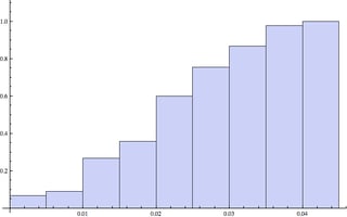
If I generate histograms for this data it looks like this:

Column[{
    Histogram[data, {.005}, "Probability", ImageSize -> Large], 
    Histogram[data, {0.005}, "CDF", ImageSize -> Large]
}]
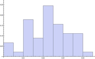
PDF CDF

My question is twofold.

  1. Is there a way to "fit" this data with a distribution? Or make a pseudo-distribution with this data? I've found d = EmpiricalDistribution[data]; DiscretePlot[CDF[d, x], {x, 0, .05, .0001}], but is this the best way?

  2. How do you programmatically calculate the P50 value from this data? (50% confidence that the value will be realized. y = 0.5 on CDF plot)

$\endgroup$
4

1 Answer 1

22
$\begingroup$

There are basically four ways you can do this:

  1. Discretely, using EmpiricalDistribution, as you suggest in your question
  2. Also discretely, but in a bucketed way, using HistogramDistribution
  3. Smoothly, using SmoothKernelDistribution or KernelMixtureDistribution.
  4. By fitting an assumed distribution, e.g. by using EstimatedDistribution, FindDistributionParameters and related commands.

Which you choose depends on the nature of your data and what you know about it. If you have reason to believe the data are distributed according to some known distribution, choose #4. Since your data are real-valued, it is likely that it comes from a continuous distribution and so choices #3 or #4 seem most appropriate.

Once you have your estimated distribution, you can calculate the P50 value using Quantile.

It is worth noting, though, that particular settings will give different estimates of the quantile. For example there is more than one way to define the kernel used in SmoothKernelDistribution. Using the data in your question:

Quantile[SmoothKernelDistribution[data ,  Automatic, #], 0.5] & /@
 {"Biweight", "Cosine", "Epanechnikov", "Gaussian", 
  "Rectangular", "SemiCircle", "Triangular", "Triweight"}

{0.0222671, 0.0223012, 0.0223522, 0.0223533, 0.0223458, 0.0223374,  0.0222653, 0.0222342}

Of course, in some fields, four decimal places is close enough.

$\endgroup$
4
  • 1
    $\begingroup$ "...using Quantile[]." - or InverseCDF[]. $\endgroup$ Commented Aug 30, 2012 at 1:44
  • $\begingroup$ @Verbeia, Thanks for the answer. And yes, I usually work on stuff a mile or more underground, 4 decimals is plenty. $\endgroup$
    – kale
    Commented Aug 30, 2012 at 2:08
  • $\begingroup$ @kale - you are most welcome. I count my own field (economics) as one where four significant figures is plenty. Indeed, more than three or four usually invites mockery and (justified) jibes of providing false precision. $\endgroup$
    – Verbeia
    Commented Aug 30, 2012 at 2:16
  • $\begingroup$ @Verbeia, in addition to SmoothKernelDistribution, Quantile itself has a 4-dimensional parameter space (so much for "non-parameteric") that is not well-documented. Certain points in this parameter space are associated with named methods, but it's difficult to relate them or interpolated values. $\endgroup$ Commented Aug 30, 2012 at 15:14

Your Answer

By clicking “Post Your Answer”, you agree to our terms of service and acknowledge you have read our privacy policy.

Not the answer you're looking for? Browse other questions tagged or ask your own question.