13
$\begingroup$

I wrote a function called deBoor using the Cox-de Boor algorithm to generate a B-spline curve.

(*Search the index of span [ui,ui+1)*)
searchSpan[knots_, u0_] :=
 With[{max = Max[knots]},
  If[u0 == max,
   Position[knots, max][[1, 1]] - 2,
   Ordering[UnitStep[u0 - knots], 1][[1]] - 2]
]
(*The definition of α coefficient*)
α[{deg_, knots_}, {j_, k_}, u0_] /; 
  knots[[j + deg + 2]] == knots[[j + k + 1]] := 0
α[{deg_, knots_}, {j_, k_}, u0_] := 
  (u0 - knots[[j + k + 1]])/(knots[[j + deg + 2]] - knots[[j + k + 1]])

(*Implementation of de Boor algorithm*)
deBoor[pts : {{_, _} ..}, {deg_, knots_}, u0_] := 
 Module[{calcNextGroup, idx = searchSpan[knots, u0]},
  calcNextGroup =
   Function[{points, k},
    Module[{coords, coeffs},
     coords = Partition[points, 2, 1];
     coeffs = {1 - #, #} & /@ (α[{deg, knots}, {#, k + 1}, u0] & /@
      Range[idx - deg, idx - k - 1]);
     {Plus @@@ MapThread[Times, {coords, coeffs}], k + 1}]
  ];
  Nest[calcNextGroup[Sequence @@ #] &,
   {pts[[idx - deg + 1 ;; idx + 1]], 0}, deg][[1, 1]]
]

TEST

points = 
 {{1, 4}, {.5, 6}, {5, 4}, {3, 12}, {11, 14}, {8, 4}, {12, 3}, {11, 9}, {15, 10}, {17, 8}};
(*here, I set the knots uniformly*)
knots = {0, 0, 0, 0, 1/7, 2/7, 3/7, 4/7, 5/7, 6/7, 1, 1, 1, 1};

ParametricPlot[
  deBoor[points, {3, knots}, t], {t, 0, 1}, Axes -> False]
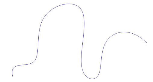
enter image description here

Now, I need to close this curve. My first thought is append the first point to the pts list.

pointsCLOSE = 
 {{1, 4}, {.5, 6}, {5, 4}, {3, 12}, {11, 14}, {8, 4}, {12, 3}, 
  {11, 9}, {15, 10}, {17, 8}, {1, 4}};
(*here, I set the knots uniformly*)
knotsCLOSE = {0, 0, 0, 0, 1/8, 2/8, 3/8, 4/8, 5/8, 6/8, 7/8, 1, 1, 1, 1};
ParametricPlot[
 deBoor[pointsCLOSE, {3, knotsCLOSE}, t], {t, 0, 1}, Axes -> False]
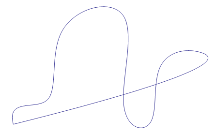
enter image description here

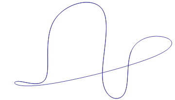
However, the built-in BSplineCurve gives a different curve

Graphics[{BSplineCurve[points, SplineClosed -> True]}]
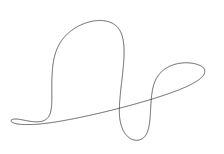
enter image description here

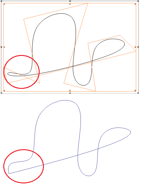
The comparison of two graphics

enter image description here

So my thought is wrong

In the chat room, thanks to halirutan's suggestion

For this closed form, you need to assume the endpoints to be periodic. It is not enough to just pre-/append one point.

QUESTION

  • What does the the endpoints to be periodic mean? I didn't learn it from The NURBS Book

  • How to generate a closed B-spline curve like the built-in BSplineCurve[pts, SplineClosed -> True] ?

UPDATE

uniformKnots[pts_, deg_] :=
 With[{n = Length@pts},
  Join[
   ConstantArray[0, deg + 1],
   Range[1, n - deg - 1]/(n - deg),
   ConstantArray[1, deg + 1]]
  ]

Manipulate[
 With[{pts = Join[points, points[[1 ;; n]]]},
  ParametricPlot[
   deBoor[pts, {3, uniformKnots[pts, 3]}, t], {t, 0, 1}, 
   Axes -> False]], {n, 1, 10, 1}
]
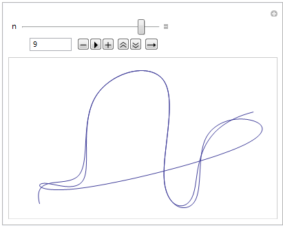
enter image description here

  • I didn't how many points should I append to the original points list?
$\endgroup$
5
  • $\begingroup$ I think you can think of endpoint-periodic like the PeriodicInterpolation for Interpolation. $\endgroup$
    – Silvia
    Commented Sep 1, 2015 at 2:45
  • $\begingroup$ @Silvia, thanks a lot :) According to your hint, I copy the entire points to the last position of pts list. Namely, pointsCLOSE1 = {{1, 4}, {.5, 6}, {5, 4}, {3, 12}, {11, 14}, {8, 4}, {12, 3}, {11, 9}, {15, 10}, {17, 8}, {1, 4}, {.5, 6}, {5, 4}, {3, 12}, {11, 14}, {8, 4}, {12, 3}, {11, 9}, {15, 10}, {17, 8}}; knotsCLOSE1 = {0, 0, 0, 0, 1/17, 2/17, 3/17, 4/17, 5/17, 6/17, 7/17, 8/17, 9/17, 10/17, 11/17, 12/17, 13/17, 14/17, 15/17, 16/17, 1, 1, 1, 1};ParametricPlot[deBoor[pointsCLOSE1, {3, knotsCLOSE1}, t], {t, 0, 1}, Axes -> False] $\endgroup$
    – xyz
    Commented Sep 1, 2015 at 3:05
  • 1
    $\begingroup$ @Silvia which gernerates a curve like built-in, please see here Obviously, the entire points that adding to the last posotion is too many. I would like to know how many points did I need to add? THX:) $\endgroup$
    – xyz
    Commented Sep 1, 2015 at 3:05
  • $\begingroup$ Good to know :) Though I think there should be easier way by manipulating the knots' weights. $\endgroup$
    – Silvia
    Commented Sep 1, 2015 at 3:07
  • $\begingroup$ @Silvia, The knotssequence own this style $\{u_0, u_1,\cdots,u_m\}$, points own the style $\{P_0,P_1,\cdots,P_n\}$. In addtion the degree of B-spline curve is $p$, so they own the following relationship $$n+1+p=m$$ In general, the knots is uniform. $\endgroup$
    – xyz
    Commented Sep 1, 2015 at 3:14

2 Answers 2

11
$\begingroup$

The following works for your curve:

points = {{1, 4}, {.5, 6}, {5, 4}, {3, 12}, {11, 14}, {8, 4}, {12, 3}, {11, 9},
          {15, 10}, {17, 8}};
deg = 3; 
pointsCLOSE1 = Join[points, points];
n = Length@pointsCLOSE1;
knotsCLOSE1 = Range[0, 1, 1/(n + 1)];
ParametricPlot[deBoor[pointsCLOSE1, {deg, knotsCLOSE1}, t], {t, deg/(n + 1), 1}, 
               Axes -> False]

Mathematica graphics

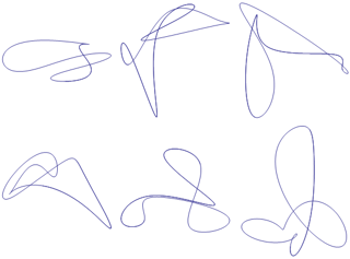
And also for many other curves

curve[nPts_, deg_] := Module[{points, pointsCLOSE1, n, knotsCLOSE1},
  points = RandomReal[{0, 1}, {nPts, 2}]; 
  pointsCLOSE1 = Join[points, points];
  n = Length@pointsCLOSE1;
  knotsCLOSE1 = Range[0, 1, 1/(n + 1)];
  ParametricPlot[ deBoor[pointsCLOSE1, {deg, knotsCLOSE1}, t], 
                  {t, deg/(n + 1), 1}, Axes -> False]
  ]

degs = RandomInteger[{3, 6}, 6];
npoints = RandomInteger[{2 #, 3 #}] & /@ degs;
Partition[MapThread[curve, {npoints, degs}], 3] // Grid

Mathematica graphics

But I've also found some counterexamples, so it should be taken with care ...

$\endgroup$
5
  • $\begingroup$ About the NURBS, in general, for a curve of degree $p$, the knots owns the following style $$\{u_0,\cdots,u_p,u_{p+1},\cdots, u_{m-p},\cdots, u_m\}$$ where $u_0=\cdots=u_p=0$ and $u_{m-p}=\cdots=u_m=1$. So I'd like to know why you set the knots to Range[0, 1, 1/(n + 1)] and changed the interval to [deg/(n + 1), 1]. THX a lot:) $\endgroup$
    – xyz
    Commented Sep 1, 2015 at 9:26
  • $\begingroup$ @ShutaoTang I tried a few things until it worked. Sorry, zero NURBS knowledge here :) $\endgroup$ Commented Sep 1, 2015 at 14:42
  • $\begingroup$ I would like to know what method did you used to achieve the right result. Especially for the setting knotsCLOSE1 = Range[0, 1, 1/(n + 1)]; and {t, deg/(n + 1), 1}, very apperciate it:) $\endgroup$
    – xyz
    Commented Sep 2, 2015 at 2:49
  • 1
    $\begingroup$ @ShutaoTang Just luck. I made a cursory browse at a few web pages about NURBS and thought that those may work. Anyway, I'm sure that it isn't completely right. I made up some examples resulting in open curves $\endgroup$ Commented Sep 2, 2015 at 3:40
  • $\begingroup$ I cannot understand this sentenceWrap the first $p$ and last $p$ control points $\endgroup$
    – xyz
    Commented Sep 2, 2015 at 11:11
3
$\begingroup$

I seem to have missed this earlier. Anyway, creating a closed spline in Mathematica explicitly is actually rather simple. Witness the following:

pts = {{1, 4}, {.5, 6}, {5, 4}, {3, 12}, {11, 14}, {8, 4}, {12, 3}, {11, 9},
       {15, 10}, {17, 8}};

m = 5; (* degree *) n = Length[pts];
f = BSplineFunction[pts, SplineClosed -> True, SplineDegree -> m];

fn = BSplineFunction[ArrayPad[pts, {{0, m}, {0, 0}}, "Periodic"], 
                     SplineDegree -> m, 
                     SplineKnots -> ArrayPad[Subdivide[n], m, "Extrapolated"]];

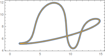
See the correspondence:

ParametricPlot[{f[t], fn[t]}, {t, 0, 1}, Axes -> None, Frame -> True, 
               PlotStyle -> {AbsoluteThickness[6], AbsoluteThickness[2]}]

matched periodic splines

Further proof of correspondence can be seen by trying ParametricPlot[f[t] - fn[t], {t, 0, 1}].

Another example:

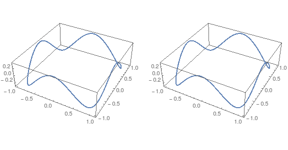
pts = {{0, 1, 1}, {1, 1, -1}, {1, 0, 1}, {1, -1, -1}, {0, -1, 1}, {-1, -1, -1},
       {-1, 0, 1}, {-1, 1, -1}};
n = Length[pts];
f = BSplineFunction[pts, SplineClosed -> True];
fn = BSplineFunction[ArrayPad[pts, {{0, 3}, {0, 0}}, "Periodic"], 
                     SplineKnots -> ArrayPad[Subdivide[n], 3, "Extrapolated"]];

{ParametricPlot3D[f[t], {t, 0, 1}], ParametricPlot3D[fn[t], {t, 0, 1}]}
// GraphicsRow

two identical 3D B-splines

$\endgroup$
5
  • 1
    $\begingroup$ Thanks J.M. In fact, I known the BSplineCurve[pts, SplineClosed -> True] could generate a closed B-spline. Firstly, I tried the method mentioned here。 However, it failed. I understood the theory of closed B-spline until I read the section 12.2 of The NURBS Book occasionally. $\endgroup$
    – xyz
    Commented Oct 9, 2015 at 7:50
  • $\begingroup$ Right, so pay attention to what I did to the knots and control points. :) $\endgroup$ Commented Oct 9, 2015 at 8:12
  • $\begingroup$ Yes, I have attentioned the control points and knots that you specified in BSplineFunction. BTW, how did you know the control points and knotsthat generating a closed B-spline? Namely, I would like to know which paper or textbook describes this in detail. :) $\endgroup$
    – xyz
    Commented Oct 9, 2015 at 8:24
  • $\begingroup$ I'll need to look up which refs have them; will ping you as soon as I find them. $\endgroup$ Commented Oct 9, 2015 at 9:37
  • $\begingroup$ Ah, there... the uniform knot vector presented in Shutao's answer and this answer seems a bit... different. His solution extrapolates only at the end; mine extends both the beginning and the end of the uniform knot vector. I suppose they are equivalent up to scaling, tho. $\endgroup$ Commented Oct 18, 2015 at 14:30

Your Answer

By clicking “Post Your Answer”, you agree to our terms of service and acknowledge you have read our privacy policy.

Not the answer you're looking for? Browse other questions tagged or ask your own question.