I have some points in 3D space that I want to plot as a closed surface. My data is at the bottom of this post.
I tried with ListPlot3D but I got something I don't want:
ListPlot3D[data]
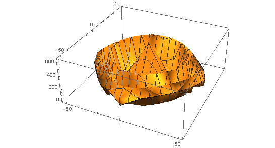
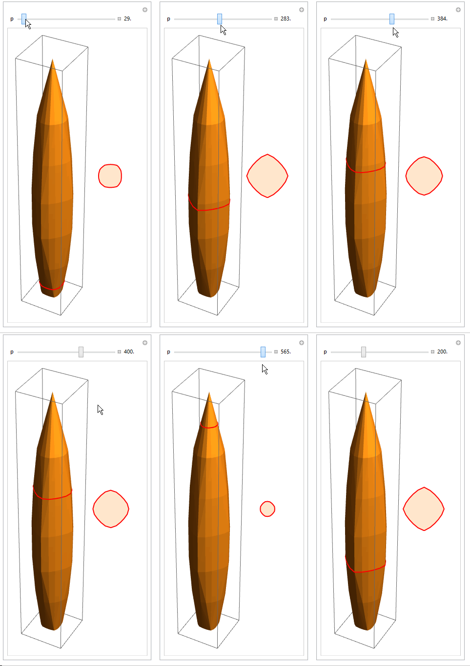
I want it to look like an ellipsoid, a closed surface... with ListPointPlot3D you can see the shape I'm looking for:
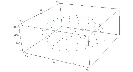
Also, if you can help me make the plot a little smooth and maybe a bit transparent, that would be awesome.
Here's the data:
data = {{0., 0., 641.096}, {0., 0., 641.096}, {0., 0., 641.096}, {0., 0.,
  641.096}, {0., 0., 641.096}, {0., 0., 641.096}, {0., 0.,
  641.096}, {0., 0., 641.096}, {0., 0., 641.096}, {0., 0.,
  641.096}, {0., 0., 641.096}, {0., 0., 641.096}, {0., 0.,
  641.096}, {0., 0., 641.096}, {0., 0., 641.096}, {0., 0.,
  641.096}, {0., 0., 641.096}, {0., 0., 641.096}, {0., 0.,
  641.096}, {0., 0., 641.096}, {0., 0.,
  641.096}, {-33.4358, -0.000480308, 500.}, {-32.4323, -10.5379,
  500.}, {-26.8297, -19.4933, 500.}, {-19.7593, -27.1967,
  500.}, {-10.91, -33.5769, 500.}, {0.0000221887, -34.9043,
  500.}, {10.7511, -33.0892, 500.}, {19.4879, -26.8225,
  500.}, {26.5746, -19.3074, 500.}, {32.4483, -10.5432,
  500.}, {33.779, -0.000441205, 500.}, {32.4484, 10.543,
  500.}, {26.5744, 19.3075, 500.}, {19.4878, 26.8226, 500.}, {10.7517,
   33.0889, 500.}, {1.45002*10^-6, 34.9043, 500.}, {-10.9098, 33.577,
  500.}, {-19.7596, 27.1965, 500.}, {-26.8301, 19.4927,
  500.}, {-32.4323, 10.5378, 500.}, {-33.4352, 0.000440213,
  500.}, {-44.8491, -0.0000166531, 400.}, {-41.3575, -13.4379,
  400.}, {-33.6225, -24.4282, 400.}, {-24.6804, -33.9701,
  400.}, {-13.8613, -42.6607, 400.}, {-0.000099884, -46.8974,
  400.}, {13.6798, -42.102, 400.}, {24.3378, -33.4982,
  400.}, {33.2163, -24.1336, 400.}, {41.0551, -13.3398,
  400.}, {44.9359, 0.000653844, 400.}, {41.0551, 13.3396,
  400.}, {33.2166, 24.1332, 400.}, {24.3377, 33.4982, 400.}, {13.68,
  42.1019, 400.}, {-0.380491, 46.8615, 400.}, {-13.8612, 42.6607,
  400.}, {-24.6807, 33.9699, 400.}, {-33.6224, 24.4283,
  400.}, {-41.3572, 13.4384, 400.}, {-44.8703, 0.000712753,
  400.}, {-51.8426, -0.000612579, 300.}, {-45.947, -14.9298,
  300.}, {-37.0981, -26.9527, 300.}, {-27.1985, -37.4354,
  300.}, {-15.3933, -47.3767, 300.}, {0.0000437598, -54.3818,
  300.}, {15.1401, -46.5957, 300.}, {26.7232, -36.7818,
  300.}, {36.4393, -26.4748, 300.}, {45.1719, -14.6771,
  300.}, {51.3474, -0.000353001, 300.}, {45.1719, 14.6771,
  300.}, {36.4393, 26.4747, 300.}, {26.7239, 36.7812, 300.}, {15.1401,
   46.5957, 300.}, {-0.000270231, 54.3818, 300.}, {-15.3935, 47.3766,
  300.}, {-27.1984, 37.4355, 300.}, {-37.0975, 26.9534,
  300.}, {-45.9476, 14.9289, 300.}, {-51.8443, 0.000903271,
  300.}, {-52.5272, -0.00080404, 200.}, {-45.9094, -14.9169,
  200.}, {-37.0924, -26.9492, 200.}, {-27.2028, -37.4414,
  200.}, {-15.3595, -47.2722, 200.}, {-0.000200055, -54.4177,
  200.}, {15.0395, -46.2864, 200.}, {26.4513, -36.4061,
  200.}, {35.8459, -26.0443, 200.}, {44.1364, -14.3409,
  200.}, {49.9257, -0.000704932, 200.}, {44.1365, 14.3407,
  200.}, {35.8467, 26.0433, 200.}, {26.4509, 36.4065, 200.}, {15.0397,
   46.2862, 200.}, {-0.000269662, 54.4176, 200.}, {-15.3598, 47.272,
  200.}, {-27.2031, 37.4411, 200.}, {-37.0926, 26.949,
  200.}, {-45.9095, 14.9167, 200.}, {-52.5279, 0.000854614,
  200.}, {-43.4968, -0.000346691, 100.}, {-39.8229, -12.9395,
  100.}, {-32.3192, -23.4813, 100.}, {-23.4945, -32.3374,
  100.}, {-12.9069, -39.7228, 100.}, {0.0000104505, -42.204,
  100.}, {12.8085, -39.4206, 100.}, {22.7948, -31.3738,
  100.}, {30.9405, -22.4796, 100.}, {36.9038, -11.9906,
  100.}, {39.5753, -0.000198095, 100.}, {36.9038, 11.9908,
  100.}, {30.9405, 22.4796, 100.}, {22.7945, 31.374, 100.}, {12.8087,
  39.4206, 100.}, {-0.000468123, 42.2039, 100.}, {-12.9068, 39.7229,
  100.}, {-23.4949, 32.3371, 100.}, {-32.319, 23.4815,
  100.}, {-39.823, 12.9393, 100.}, {-43.4973, 0.000701222,
  100.}, {-25.4858, -0.00042188, 0.}, {-25.0489, -8.13889,
  0.}, {-22.6818, -16.4793, 0.}, {-15.9412, -21.9417,
  0.}, {-7.52493, -23.1593, 0.}, {0.0000252356, -23.3718,
  0.}, {7.47278, -22.9986, 0.}, {15.7025, -21.6126,
  0.}, {20.0976, -14.6021, 0.}, {21.0782, -6.84871, 0.}, {21.2778,
  0.000336608, 0.}, {21.0782, 6.84873, 0.}, {20.0977, 14.6019,
  0.}, {15.7025, 21.6126, 0.}, {7.47262, 22.9986, 0.}, {-0.0000887879,
   23.3719, 0.}, {-7.52488, 23.1592, 0.}, {-15.9413, 21.9416,
  0.}, {-22.6722, 16.4442, 0.}, {-25.0478, 8.14015, 0.}, {-25.4415,
  0.0941868, 0.}}

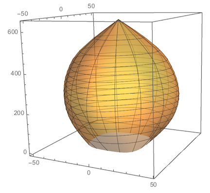
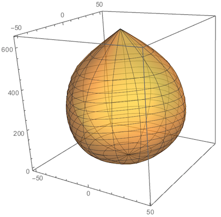


ConvexHullMesh? $\endgroup$