Developing a function of two variables from given data

Question

Cross listed from MSE: https://math.stackexchange.com/questions/1029399/developing-a-function-of-two-variables-from-given-data

(I believe Mathematica SE is an appropriate place to ask this, as well.)

I have been stuck on the following problem.

Consider a system where we have three variables: force $F$, orientation $\theta$, and temperature $T$. I want to find a function for force such that $F=f(\theta,T)$.

In this system, we choose some orientation $\theta$ and temperature $T$, and from these values we want to determine the force $F$ yielded.

We only know the force values corresponding to $\theta=$ 10, 20, 30, 40, 50 or 60 and $T=$ 200, 182, etc., as shown in the table below.

Table displaying forces $F$:

(Note: I tried to turn this into an array in $\TeX$ but I couldn't get it to work, so here's a screenshot. I realize that Mathematica users will want the data written out for copy/paste purposes--if you can help me create an array that works, I will edit this an use that array. Thanks)

Example: For $\theta=30$ and $T=164$, we found that the force $F=31.87$.

Now here's my question: How do I find a function for $F$ that can handle "in between" values for both $\theta$ and $T$?

Here's what I mean: I would like a function $F=f(\theta,T)$ for values like $\theta=34$ and $T=195$, or any values $\theta$ and $T$ that are not on the table above. However, I only need this function for the interval $\theta\in[10,60]$ and $T\in[101,200]$. Essentially, I am trying to approximate $F$ for all $\theta\in[10,60]$ and $T\in[101,200]$.

I should note that I enjoy working on problems like these, so if somebody knows the answer, please try giving hints instead of solutions so that I can figure this out myself.

I have made little progress so far. I observed that the relationship between $F$ and $\theta$ is linear, while the relationship between $F$ and $T$ is nonlinear. The latter nonlinear relationship appears to be best approximated with a 2nd order polynomial. So far, I have six different functions (polynomial fit lines) for the six different $\theta$. Any hints on how to proceed? Not really sure which field of mathematics this falls under. Please let me know if you'd like me to elaborate some more on my attempts to solve this, and I'd be happy to share.

Thank you.

Answer 1

Update, as per new requests:

Importing from xls files:

s = Part[Import["~/Downloads/s.xlsx"], 1, 1]
t = Part[Import["~/Downloads/t.xlsx"], 1, 1]
data = Part[Import["~/Downloads/data.xlsx"], 1]

(* Using @ubpdqn much nicer data massaging *)
table = Join @@ MapThread[Join[{#1}, {#2}] &, {Outer[List, s, t], data}, 2];

For the part 1) of your request: intFun is your $f(\theta, T)$, and can be used like this:

intFun = Interpolation[table];
intFun[30, 180]

30.94

For the part 2) of your request: the table of all force $F$ for the specified $\theta$ and $T$, with 0.5 and 1 increments, respectively.

finalTable = Table[Table[intFun[s1, t1], {t1, Max@t, Min@t, -1}], {s1, Min@s, Max@s, 0.5}]

{{3.80765,3.79107,3.77423,3.75713,3.73976,3.72211,3.70417,3.68594,3.66742,3.64858,3.62942,...105...,0.588854,0.577435,0.559586,0.5445,0.524866,0.493372,0.442709,0.410001,0.392214,0.386318,0.389277},...129...,{...1...}}

Previous answer

Using some made up data with the trends you mentioned:

data = Table[Table[{{o, t}, o + 3 t/120 + RandomReal[{-1, 1}]}, {t, 200, 80, -20}], {o, 10, 60, 10}];

You can ask Mathematica to do all the hard work for you, and interpolate the data using splines or Hermite interpolation

int = Interpolation[Flatten[data, 1]]

InterpolatingFunction[{{10., 60.}, {80., 200.}}, <>]

int is your $f(\theta, T)$, and can be used like this:

Plot[int[35, x], {x, 0, 300}]
Plot[int[x, 110], {x, 0, 100}]

You can also extrapolate values (as above), but it warns you that it is doing so, and the first plot shows exactly why.

If you have some good guesses about the underlying model, you can always try to fit the parameters. In your case, $a + b *\theta + c *T + d *t^2$

(* Massaging data back to triples *)
data2 = Flatten /@ Flatten[data, 1]

(* A model of the form a + b*o + c*t + d*t^2 *)
model = Fit[data2, {1, o, t, t^2}, {o, t}]

0.941482 + 1.00358 o + 0.00545877 t + 0.0000743324 t^2

This model can be used as:

model./{o->value1, t->value2}

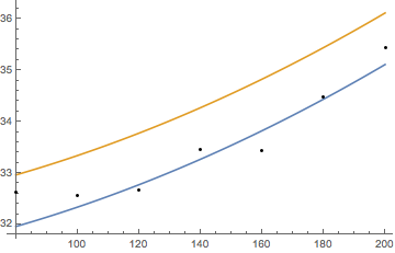
Plot[{model /. o -> 30, model /. o -> 31}, {t, 80, 200}, Epilog -> Point@Cases[data2, {30, t_, f_} :> {t, f}]]

Blue for $\theta=30$, along with the corresponding data points

Orange for $\theta=31$

Answer 2

Using Mathematica version 10 new Predict Function

t = {200, 182, 164, 146, 128, 110, 101, 92, 83}; 
s = {10, 20, 30, 40, 50, 60};
data = {{10.24, 10.15, 10.01, 9.81, 9.39, 8.8, 8.57, 7.89, 7.23},
{21.50, 21.52, 21.25, 20.88, 20.79, 20.66, 20.37, 19.98, 19.50},
{31.92, 32.09, 31.87, 31.58, 31.31, 30.99, 30.86, 30.87, 30.41}, 
{43.56, 43.88, 43.63, 43.29, 43.02, 42.57, 42.16, 42.52, 42.25}, 
{54.85, 55.28, 54.98, 54.57, 54.36, 54.07, 53.78, 54.03, 54.12}, 
{64.45, 65.01, 64.78, 64.46, 64.36, 64.20, 63.94, 64.10, 64.54}};
vals = Flatten[Table[{s[[i]], t[[j]], data[[i, j]]}, {i, Length@s}, {j, Length@t}],1]
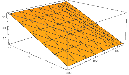
ListPlot3D[vals, Mesh -> All]

It is a plane, we can use linear regression as the method for the Predict Function

Set up the training set now and get the predictor function.

trainingSet = Flatten[Table[Rule[{s[[i]], t[[j]]}, data[[i, j]]], {i, Length@s}, {j, 
Length@t}], 1];
pf = Predict[trainingSet, Method -> "LinearRegression"];
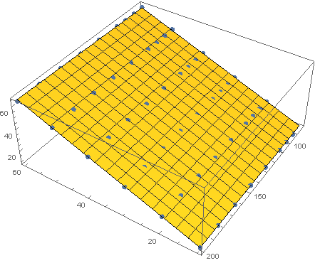
Show[Plot3D[pf[{x, y}], {x, Min@s, Max@s}, {y, Min@t, Max@t}], 
ListPointPlot3D[vals, PlotStyle -> {PointSize -> Large}]]

Let's get the function now.

PredictorInformation[pf, "Function"]
(*-3.62101 + 1.11233 #1 + 0.0138794 #2 &*)

Please read the documentation on Predict, PredictorFunction and PredictorMeasurements.

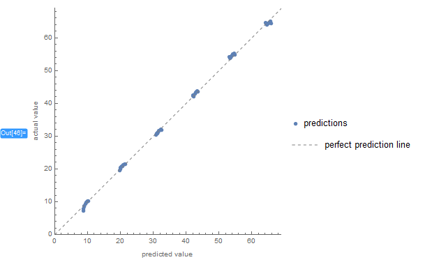
Some cool functionality.

PredictorMeasurements[pf, testSet, "ComparisonPlot"]

UPDATE

With the new dataset provided via Dropbox, the use of Predict is not the right approach.

First Step is to import the data

data = Import[
  "https://www.dropbox.com/s/v3c8kngvohgf62m/data.xlsx?dl=1", {"Data",
    1}];
s = Import[
   "https://dropbox.com/s/30hx04aszlafgk7/s.xlsx?dl=1", {"Data", 
    1}][[1]];
t = Import[
   "https://dropbox.com/s/ijkyuley8q3830p/t.xlsx?dl=1", {"Data", 
    1}][[1]];

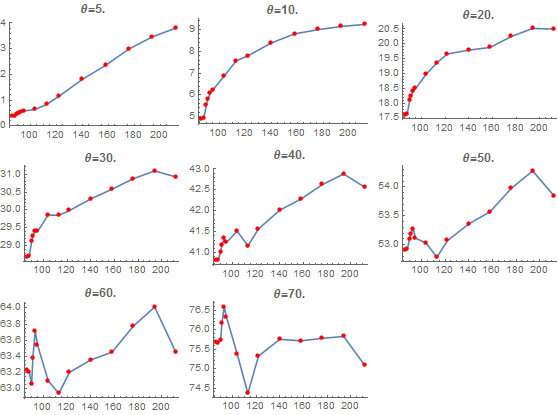
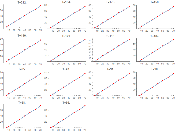
Second step is to visualize the information. Check the data in the 2 different axes.

vals = Table[{s[[i]], t[[j]], data[[i, j]]}, {i, Length@s}, {j, 
    Length@t}];
Multicolumn[
 ListPlot[vals[[#, All, 2 ;;]], Joined -> True, 
    PlotMarkers -> Graphics[{Red, PointSize[Medium], Point[{0, 0}]}], 
    PlotLabel -> 
     Style[StringJoin["\[Theta]=", ToString[s[[#]]]], Bold]] & /@ 
  Range@Length@s, {Automatic, Automatic}, Appearance -> "Horizontal"]

Multicolumn[(ListPlot[vals[[All, #1, {1, 3}]], Joined -> True, 
      PlotMarkers -> 
       Graphics[{Red, PointSize[Medium], Point[{0, 0}]}], 
      PlotLabel -> Style["T=" <> ToString[t[[#1]]], Bold]] &) /@ 
   Range[Length[t]], {Automatic, Automatic}, 
  Appearance -> "Horizontal"]]

trainingSet = 
  Flatten[Table[{{s[[i]], t[[j]]}, data[[i, j]]}, {i, Length@s}, {j, 
     Length@t}], 1];
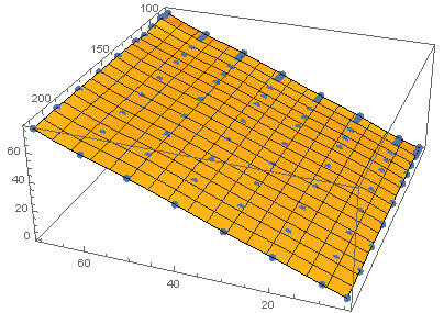
pf = Interpolation[trainingSet]
Show[Plot3D[pf[x, y], {x, Min@s, Max@s}, {y, Min@t, Max@t}], 
 ListPointPlot3D[vals, PlotStyle -> {PointSize -> Large}]]

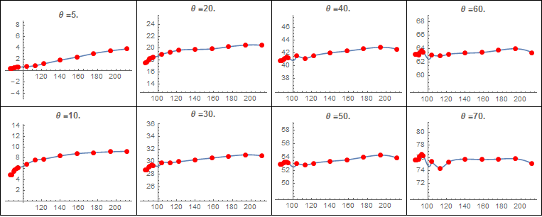
Check one axes

Multicolumn[
 Plot[pf[#, x], {x, Min@t, Max@t}, PlotRangePadding -> 5, 
    Epilog -> {Red, PointSize[Large], 
      Point[Flatten[Cases[vals, {{#, _, _} ..}], 1][[All, 2 ;;]]]}, 
    PlotLabel -> 
     Style[StringJoin["\[Theta] =", ToString[#]], Bold]] & /@ s, {2, 
  Automatic}, Frame -> All, Appearance -> Vertical]

Answer 3

Setup:

data = {{10.24, 10.15, 10.01, 9.81, 9.39, 8.8, 8.57, 7.89, 
    7.23}, {21.50, 21.52, 21.25, 20.88, 20.79, 20.66, 20.37, 19.98, 
    19.50}, {31.92, 32.09, 31.87, 31.58, 31.31, 30.99, 30.86, 30.87, 
    30.41}, {43.56, 43.88, 43.63, 43.29, 43.02, 42.57, 42.16, 42.52, 
    42.25}, {54.85, 55.28, 54.98, 54.57, 54.36, 54.07, 53.78, 54.03, 
    54.12}, {64.45, 65.01, 64.78, 64.46, 64.36, 64.20, 63.94, 64.10, 
    64.54}};
t = {200, 182, 164, 146, 128, 110, 101, 92, 83};
s = {10, 20, 30, 40, 50, 60}; pts = 
 MapThread[Join[{#1}, {#2}] &, {Outer[List, s, t], data}, 2];
pt = MapThread[Join[#1, {#2}] &, {Outer[List, s, t], data}, 2];

You can use Interpolation:

if = Interpolation[Join @@ pts];
int = Show[
   Plot3D[if[x, y], {x, 10, 60}, {y, 83, 200}, PlotStyle -> LightPink,
     Mesh -> None], 
   Graphics3D[{Red, PointSize[0.02], Point[Join @@ pt]}], 
   ImageSize -> 200];

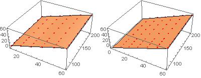
or LinearModelFit (similar to Predict` as per PatoCriollo):

lr = LinearModelFit[Join @@ pt, {1, x, y}, {x, y}];
reg = Show[
   Plot3D[lr[x, y], {x, 0, 60}, {y, 80, 200}, Mesh -> False, 
    PlotStyle -> LightPink], 
   Graphics3D[{Red, PointSize[0.02], Point[Join @@ pt]}], 
   ImageSize -> 200];

The left plot below is interpolated surface, the right linear regression plane: