6
$\begingroup$

I created a spline function from a list of points and made a plot as follows:

  list2 = {{3.93453, -0.623168}, {3.79708, -0.187231}, {3.72835, 
  0.0307369}, {3.65963, 0.248705}, {3.5909, 0.466673}, {3.52218, 
  0.684642}, {3.44186, 1.05816}, {3.36155, 1.29764}, {3.28124, 
  1.5219}, {3.20093, 1.73094}, {3.12061, 1.92474}, {3.0403, 
  2.10331}, {2.95999, 2.26666}, {2.87968, 2.41477}, {2.79937, 
  2.54766}, {2.71905, 2.66532}, {2.63874, 2.76774}, {2.55843, 
  2.85494}, {2.41254, 2.97924}, {1.98589, 3.2791}, {1.52249, 
  3.51828}, {1.27967, 3.61368}, {1.03092, 3.69235}, {0.777399, 
  3.75392}, {0.520275, 3.7981}, {0.260741, 3.82469}, {0., 3.83357}}

g = BSplineFunction[list2, 
      SplineWeights -> {50, 50, 50, 50, 50, 50, 50, 50, 50, 50, 50, 50, 
        50, 50, 50, 50, 50, 50, 50, 50, 50, 50, 50, 50, 50, 50, 50}]

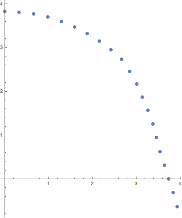
ListPlot[Table[g[t], {t, 0, 1, 1/100}]]

I need my plot to have more evenly placed points. When I take the plot out of this sample table to a larger scale plot, there are gaping holes that are too extreme for my needs. Is there any way to adjust the density of my spline function without just adding more points? Adding more points is not proving to be an effective solution.

$\endgroup$
10
  • 1
    $\begingroup$ So you want an arc-length reparametrization ... $\endgroup$ Commented Jul 14, 2014 at 22:00
  • $\begingroup$ some of this may be useful mathematica.stackexchange.com/questions/50581/… $\endgroup$
    – george2079
    Commented Jul 15, 2014 at 2:59
  • $\begingroup$ Strongly related: mathematica.stackexchange.com/q/39394 The answers there may be applied to plotting g[t]. $\endgroup$
    – Michael E2
    Commented Jul 15, 2014 at 3:18
  • 1
    $\begingroup$ @Kaisey You have asked 13 questions and accepted none of the answers. (Are they all wrong?) You should see a check mark you can click below the vote count. Accepting the best correct answer is the way such answers are marked on the site and an expected way to say "thank you" to those you tried help you. $\endgroup$
    – Michael E2
    Commented Jul 30, 2014 at 16:37
  • 1
    $\begingroup$ @Mr.Wizard I am in mixed feeling which question(s) should be closed: this thread is the only one where the general case of AspectRatio not being Automatic is considered (and in all answers!). If someone comes with another solution which takes into account the general case, this thread is the best place to post such an answer. $\endgroup$ Commented Oct 30, 2014 at 9:39

2 Answers 2

5
$\begingroup$

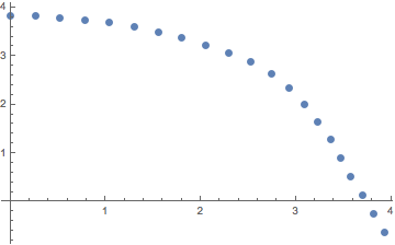
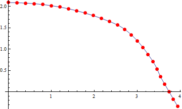
Here is an arc-length reparametrization in terms of a function tfn that maps the arclength along the B-spline curve to the parameter t. It's important to use AspectRatio -> Automatic to get the spacing even.

There are two truncation-error issues with parametrizing the full length of the curve. One is that the stopping point is found by stepping past the end of the curve. BSplineFunction does not extrapolate, so I extended its derivative in dg.The other is actually getting to the end of the curve. I dealt with it by over estimating the arclength and using WhenEvent to stop the integration. The NIntegrate used to get the total arclength is fast, so it is not very wasteful in this case. If NIntegate were slower, one could overestimate the arclength in other ways, e.g. from list2.

The domain of tfn runs from 0 to the arclength. To get even spacing, I rescaled an even division of the unit interval to the domain of tfn.

ClearAll[s, t];
(* g defined as in OP *)
dg[t_?NumericQ] := If[t - 1. <= 0, g'[t], g'[1]];
tfn = NDSolveValue[{t'[s] == 1/Norm[dg[t[s]]], t[0] == 0, 
   WhenEvent[t[s] == 1, "StopIntegration"]},
  t, {s, 0, 1 + NIntegrate[Norm[g'[t]], {t, 0, 1}]}];

ListPlot[g /@ tfn[Rescale[Range[0, 1, 1/20], {0, 1}, First@tfn["Domain"]]],
 AspectRatio -> Automatic]

Mathematica graphics

Aspect ratio

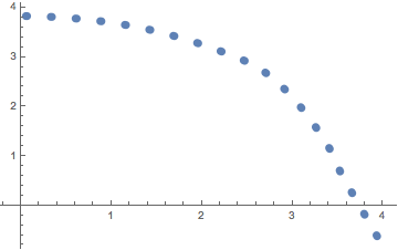
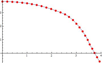
If you want a different aspect ratio other than Automatic, such as the default 1/GoldenRatio, then we have to adjust how the arclength is computed by scaling the derivative vector, e.g., by {1, 1/GoldenRatio}.

ClearAll[s, t];
(* g defined as in OP *)
dg2[t_?NumericQ] :=  If[t - 1. <= 0, g'[t], g'[1]] {1, 1/GoldenRatio};
tfn2 = NDSolveValue[{t'[s] == 1/Norm[dg2[t[s]]], t[0] == 0, 
   WhenEvent[t[s] == 1, "StopIntegration"]},
  t, {s, 0, 1 + NIntegrate[Norm[dg2[t]], {t, 0, 1}]}]

ListPlot[g /@ tfn2[Rescale[Range[0, 1, 1/20], {0, 1}, First@tfn2["Domain"]]]]

Mathematica graphics


Here is another way based on my answer to this question:

Different MeshStyle for different functions

It used to not work on Windows, but I'm not sure about whether that is so for V10.

ParametricPlot[g[t], {t, 0, 1}, 
 PlotStyle -> {Directive[CapForm["Round"], Dashing[{0, 0.06}], 
    Thickness[0.02]], Directive[]}, AspectRatio -> 1/GoldenRatio]

Mathematica graphics

$\endgroup$
2
  • $\begingroup$ Michael, please tell me (or just vote) if you believe this question can be closed as a duplicate of one of the ones linked in my comment below it. $\endgroup$
    – Mr.Wizard
    Commented Apr 15, 2015 at 17:57
  • $\begingroup$ Pay attention that the derivative of a rational B-Spline (i.e. non-trivial weights) is wrong in Mathematica. See this question mathematica.stackexchange.com/questions/214061/… $\endgroup$
    – johk95
    Commented Feb 3, 2020 at 20:29
9
$\begingroup$

As Ulises Cervantes Pimentel uncovered in this Wolfram Community thread,

Plot and ParametricPlot/ParametricPlot3D for curves can take as MeshFunctions the values "ArcLength" and "CurveLength".

This functionality provides straightforward solution for the plots with AspectRatio -> Automatic:

mpoints = Table[t, {t, 0, 1, 0.04}];
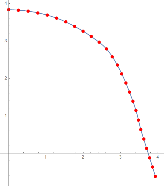
ParametricPlot[g[t], {t, 0, 1}, MeshFunctions -> {"ArcLength"}, 
 Mesh -> {mpoints}, MeshStyle -> {PointSize[0.02], Red}]

plot

The case of AspectRatio not being Automatic is more difficult. The actual ratio between the scales of the axes is determined by the FrontEnd and cannot be obtained without some kind of rendering. Below I show how the actual ratio can be obtained when the target Export format is "PDF". The output is from MMa 8.0.4 but the code works also in v. 10.0.1.

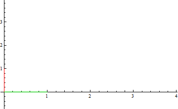
First of all, I add markers to the graphics: vertical Red and horizontal Green line and replace all the colors inside of the graphics by White:

gr = ParametricPlot[g[t], {t, 0, 1}, AspectRatio -> 1/GoldenRatio];
grWithMarkers = 
 Show[gr /. _RGBColor | _Hue -> White, 
  Epilog -> {Red, Line@{{0, 0}, {0, 1}}, Green, Line@{{0, 0}, {1, 0}}}]

plot with markers

Now I Export obtained graph to PDF and Import it backward:

grData = ImportString[ExportString[grWithMarkers, "PDF"], "PDF", 
    "TextOutlines" -> False][[1, 1]];

In the PDF's internal coordinate system the scales along the horizontal and vertical directions are identical, hence I can easily calculate the ratio in question from the lengths of the lines:

xScale = Cases[grData, 
    Style[cur_, ___, RRGBColor[0., _?Positive, 0., _], ___] :> 
     EuclideanDistance @@ cur[[1, 2, 1]], Infinity][[1]];
yScale = Cases[grData, 
    Style[cur_, ___, RGBColor[_?Positive, 0., 0., _], ___] :> 
     EuclideanDistance @@ cur[[1, 2, 1]], Infinity][[1]];
ratio = yScale/xScale

0.5456134338588072`

It is not equal to the AspectRatio which is equal to

1./GoldenRatio

0.6180339887498948`

Now I obtain uniform mesh in the natural coordinate system:

grScaled = 
 ParametricPlot[g[t] {1, ratio}, {t, 0, 1}, 
  MeshFunctions -> {"ArcLength"}, Mesh -> {mpoints}, 
  MeshStyle -> {PointSize[0.02], Red}]

plot

And apply post-processing for returning to the original coordinate system:

Graphics[#[[1]] /. {x_Real, y_Real} :> {x, y/ratio}, 
   Options[gr]] &@grScaled

plot

$\endgroup$
2
  • $\begingroup$ That's a new one! +1 I wonder if we really need yet another question on this topic however which IMHO only makes this fine answer harder to find. Please tell me if you feel that this can be closed as a duplicate of one of the questions linked in my comment above. $\endgroup$
    – Mr.Wizard
    Commented Oct 28, 2014 at 22:36
  • 1
    $\begingroup$ Closely related: mathematica.stackexchange.com/a/191353/280 $\endgroup$ Commented Feb 12, 2019 at 7:50

Not the answer you're looking for? Browse other questions tagged or ask your own question.