I have a homework project. I need to analyse a gambler's ruin where there are 6 possible outcomes of every wager with corresponding probabilities and payoffs and the gambler may vary the wager (say only 4 values). Am I correct in thinking the gambler's wealth (say 0 to 200 starting at 100) is a 2D random walk with unequal steps. The state space having bankroll on one axis and wager value on the other with bankroll increment determined by outcome, payoff and wager. I can easily simulate this in Excel (or Mathematica) but that won't provide the necessary ruin insight. I could do repeated simulations in Excel stopping at ruin and then derive an empirical PDF of ruin. Mathematica seems to have only 1D RW with equal steps
-
$\begingroup$ I was looking for a built in function, something analogous to DiscreteMarkovProcess, where I can then interrogate the function regarding stopping, ruin etc. Actually generating a walk (as in a single simulation realisation) is trivial, I can write a macro in excel in 5 minutes. But I am a newbie to Mma and the documentation is very dense in places. $\endgroup$– PatrickCommented Jan 28, 2014 at 8:10
-
$\begingroup$ Also your example looks like it has unit steps $\endgroup$– PatrickCommented Jan 28, 2014 at 8:13
-
$\begingroup$ And equal probabilities. I need to use 6 different probabilities and the payoffs are not all even money, hence the wealth increments are unequal. $\endgroup$– PatrickCommented Jan 28, 2014 at 8:37
-
$\begingroup$ For fixed wagers the problem is also trivial as I can construct a transition matrix to feed into DiscreteMarkovProcess with absorbing states (probability 1) at 0 and 200 corresponding to ruin and doubling wealth respectively. I can then interrogate the function to get ruin/doubling probabilities and other stuff. How do I accomplish the same thing with varying wagers. $\endgroup$– PatrickCommented Jan 28, 2014 at 8:55
-
$\begingroup$ How is the wage going to vary along the process? $\endgroup$– Dr. belisariusCommented Jan 28, 2014 at 10:44
1 Answer
Here you have a boilerplate for coding the simulation. I've filled each function with a "reasonable random" behavior for a betting game that follows your experiment description. You should customize them to fit better your simulation needs.
I can't infer from your question what are the random vars for your PDF, but the outcome from the function lets you get (I think) any statistic you may want:
allowedWagers[] := {1, 2, 3, 4};
wagerAmount[currentBankRoll_, lastResult_] := Module[{r},
                 While[(r = RandomChoice[allowedWagers[]]) > currentBankRoll]; r]

stopCondition[initialBankRoll_, currentBankRoll_] := Module[{},
  Which[
   currentBankRoll < Min@allowedWagers[], 0, (* 0 == Ruin *)
   currentBankRoll == 2 initialBankRoll,  1, (* 1 == Won *)
   True, 2                                   (* 2 == Continue *)
   ]
  ]

diceF[] := Module[{}, RandomChoice@Range@6]

payOff[dice_] := Module[{payoffs = {-1, -.5, -.2, .2, .4, 1}},(*returns the % gain/loss*)
                         payoffs[[dice]]
  ]

doWalk[initialBankRoll_] := Module[{lastResult = 1, bankRoll = initialBankRoll,
                                    walk = {}, wa, sc, lr},
  While[
   (sc = stopCondition[initialBankRoll, bankRoll]) == 2,
   (bankRoll = bankRoll + (wa=wagerAmount[bankRoll, lastResult]) payOff[lr = diceF[]];
    lastResult = lr;
    AppendTo[walk, {bankRoll, wa}])];
  Return@Append[walk, {sc}]
  ]
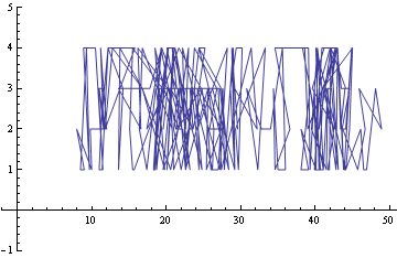
The "states space" random walk you mentioned in the question:
initialBankRoll = 20;
SeedRandom[42];
ListLinePlot[Most@doWalk[initialBankRoll], PlotRangePadding -> {2, 1}, AxesOrigin -> {0, 0}]

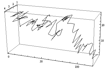
The same, viewed as a time-evolution process:
initialBankRoll = 20;
SeedRandom[42];
Graphics3D[Line@(Prepend@@@ (Transpose@{#,Range@Length@#} &@Most@doWalk[initialBankRoll])),
           BoxRatios -> {10, 5, 3}, Axes -> True]

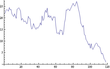
The evolution of the bank roll:
initialBankRoll = 20;
SeedRandom[42];
ListLinePlot[Most[doWalk[initialBankRoll][[All, 1]]]]

