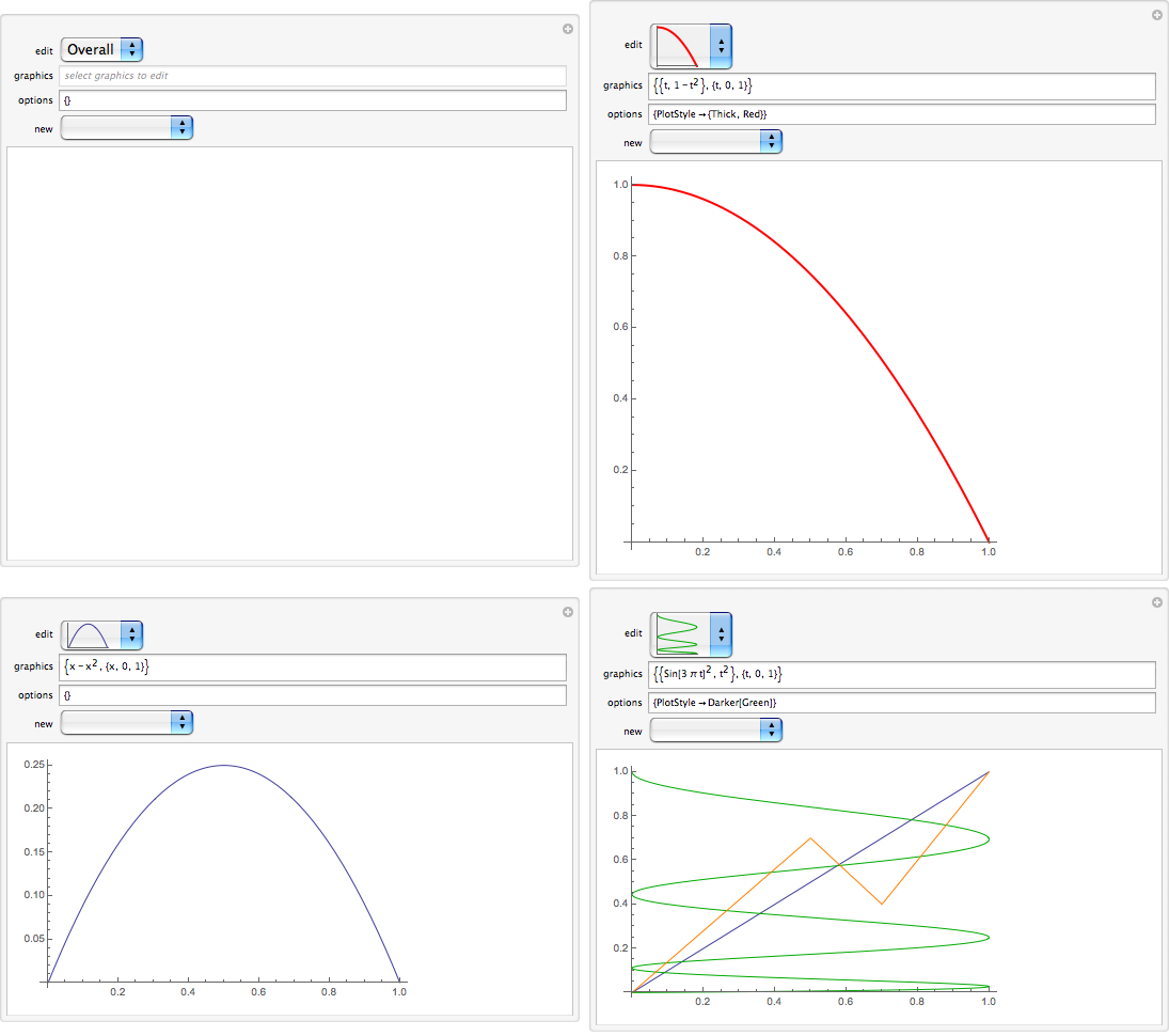
Mathematica, because of its active and dynamic capabilities, is by orders of magnitude the best method of developing and communicating technical ideas. But for various reasons it is seldom used that way. The poster is interested in better capabilities for custom plots, part of better communication, and I confine my answer to that, with a custom table also thrown in. Communication does often require extended discussion.
Mathematica has excellent underlying graphics facilities. It's weak point is in putting them together to produce custom graphics. It is difficult and confusing as opposed to natural and intuitive. This is why there are so many questions on implementing simple graphical solutions. One of the problems is that Mathematica provides many "set-piece" plots, which are nice if you are within the domain of the plot, but difficult once you stray outside. Also the method of combining plots with Show works but is rather arcane, requiring either graphics level jumping (wrapping primitives in Graphics) or the use of Epilog.
I have for a long time worked on a Mathematica Application called Presentations, which I sell for $50. It is an application designed to aid the production of custom graphics, tables, dynamic presentations, and generally literate notebooks. It has a number of essays on using Mathematica and numerous examples. It is 38 MB in size and has 511 files. It started when Version 3 appeared and, as an exercise in reviewing math and learning Mathematica, I worked all the examples and exercises and reproduced all of the graphics in the Thomas/Finney 9th Edition Calculus text. I realized then that the Mathematica paradigm was awkward and produced the first version, which I called DrawGraphics. (I since changed the name because it goes to many matters beyond graphics.)
One way of using Mathematica is to think of a notebook as blank piece of paper on which you are writing your mathematics, which other people might want to read. Similarly, we might think of a graphic as being drawn on the piece of paper, the original poster's canvas.
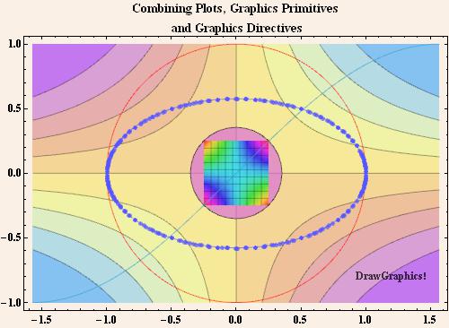
Presentations treats graphics as just drawing one thing after another where everything is a graphics primitive. It does this by providing routines, for most of the regular plot types, which extract the primitives. Here is an example, which combines a ContourPlot, a Disk, a Circle, a DensityPlot, a regular Plot, a ParametricPlot, a Contour implicit plot, the points generated by Mathematica for the implicit plot, some Text and various graphics directives. Notice that we are just drawing one thing after another.
<< Presentations`
Draw2D[
 {ContourDraw[Sin[x y], {x, -(\[Pi]/2), \[Pi]/2}, {y, -1, 1},
   ColorFunction -> ColorData["Pastel"]],
  Opacity[0.7, ColorData["Legacy", "Orchid"]],
  Disk[{0, 0}, Sqrt[2]/4],
  Black,
  Circle[{0, 0}, Sqrt[2]/4],
  DensityDraw[Sin[x y], {x, -(1/4), 1/4}, {y, -(1/4), 1/4},
   ColorFunction -> Hue, PlotPoints -> 8, Mesh -> 8],
  Draw[Sin[x], {x, -(\[Pi]/2), \[Pi]/2},
   PlotStyle -> ColorData["Legacy", "Peacock"]],
  ParametricDraw[{Cos[t], Sin[t]}, {t, 0, 2 \[Pi]},
   PlotStyle -> Red],
  ellipse = ContourDraw[x^2 + 3 y^2 == 1, {x, -1, 1}, {y, -1, 1},
    ContourStyle -> Lighter@Blue],
  Black, AbsolutePointSize[5],
  Normal[ellipse] /. Line[pts_] :> {Point[pts]},
  Black,
  Text["DrawGraphics!", Scaled[{0.95`, 0.1`}], {1, -1}]},
 Frame -> True,
 AspectRatio -> Automatic,
 Background -> ColorData["Legacy", "Linen"],
 ImageSize -> 500,
 BaseStyle -> {FontSize -> 12, FontWeight -> "Bold"},
 PlotLabel ->
  "Combining Plots, Graphics Primitives\n and Graphics Directives"]

The statement in the notebook is the record for drawing the plot. It is the most direct method and it is easy to edit and reevaluate. I would not go for any more complicated method. The various Plot statements are replaced by Draw statements. Among other things, the Draw statements have a limited set of options - only those options that actually affect the primitives being drawn. (So, for example ImageSize would not be an option that would go into a Draw statement.) On the other hand, the options that affect the overall look of the graphic go at the end. The difference between these two types of options is confusing to many users and somewhat confounded in the common use of the Show statement.
In a notebook, the graphics statement could be closed. Presentations provides an EvaluateBelowButton, which can be pasted into a Text cell preceding the graphics statement and which evaluates the cell. This way the boilerplate specifications can be at a natural place in the notebook, but hidden and, if the reader wishes, the cell can be opened to examine the code.
A graphic, such as above, could also be wrapped in a WindowPresentation routine to display it by the side of a notebook. It there is extended discussion in conjunction with the graphic then this prevents it from being scrolled out of view during the discussion.
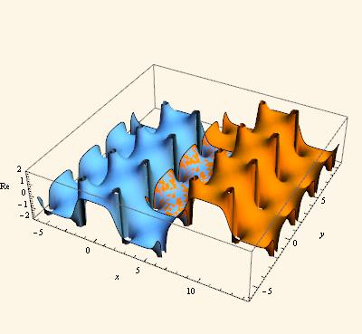
Another feature of Presentations is the recasting of the various graphics transfornations as more convenient post-fix operations. Here we demonstrate the periodicity of the JacobiCD function by superimposing a translated portion of the function on the original function. We draw and save the real part of the surface first and calculate the periods in each direction.
realsurface =
  Draw3D[Re[JacobiCD[x + I y, 2/3]], {x, -6, 6}, {y, -6, 6},
   Mesh -> None];
xperiod = 4 EllipticK[2/3] // N;
yperiod = 2 EllipticK[1 - 2/3] // N;
Then just combine the original and shifted surface. Because we are always dealing directly with the graphics primitives it is easy to not only combine but also manipulate the objects.
Draw3DItems[
 {Opacity[1, Lighter@HTML@DodgerBlue], realsurface,
  Opacity[1, Orange],
  realsurface // TranslateOp[{xperiod, yperiod, 0}]},
 NeutralLighting[0.3, 0.6, 0],
 NiceRotation,
 PlotRange -> {-2, 2},
 Axes -> True,
 AxesLabel -> {x, y, Re},
 BoxRatios -> {1, 1, 1/4},
 ImageSize -> 400]

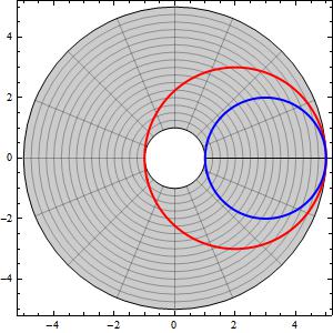
An important area of graphics is the representation of complex functions. Here it is convenient to deal directly with complex values, rather than having to squeeze everything through the x + I y filter. The following is an example. We make a plot in the complex plane and save the graphics primitives. (ComplexPolar is just a modulus/argument form of a complex number.)
Draw2D[
 {graphics2D = {DrawPolarMap[
     z, {z, ComplexPolar[1, 0], ComplexPolar[5, 2 \[Pi]]}],
    AbsoluteThickness[2],
    Red, ComplexCurve[2 + 3 E^(I \[Theta]), {\[Theta], 0, 2 \[Pi]}],
    Blue, ComplexCurve[3 + 2 E^(I \[Theta]), {\[Theta], 0, 2 \[Pi]}]}},
 Frame -> True,
 ImageSize -> 300]

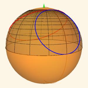
Then we map this to the Riemann sphere.
Draw3DItems[
 {ColoredRiemannSphere[],
  graphics2D // StereographicMap},
 ViewRiemann,
 ImageSize -> 300]

So I would hesitate to start designing pop-up windows and InputFields to write graphics. Graphical needs are just far too wide to design some kind of "box" to fit them into. Good graphics require detailed specification and most good graphics are unique. It is better just to have convenient routines to provide common functions and put things together. Edward Tufte, the great designer of data presentations writes: "Those who discover an explanation are often those who construct its representation." It's worth the effort.
There is, in reference to the poster's request, one pop-up item in Presentations, the OptionsFinder. (This routine was contributed by Thomas Münch and Syd Geraghty.) You can click in a name of a routine, in your code, and OptionsFinder will give a list of all the options for that routine (Mathematica routines and loaded package routines). The list will display the default option and there is a link that displays the usage message. Clicking on the link will bring up the help page for the option (if there is one). There is also a link to bring up the help page for the routine. You can also paste the option directly into your code. I use this quite a lot.
The Presentations Application also has a palette that gives quick access to all the routines, with direct links to the individual help pages, and drop-down menus for pasting templates for the various forms of commands.
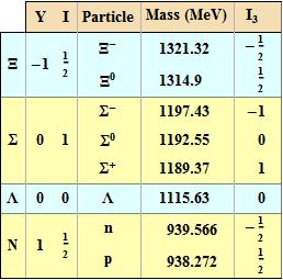
Graphics is only one example of writing literate notebooks and as a last example I would like to mention one other area - that of composing custom tables. A great deal of information is better presented in tables than with graphics. The Mathematica construct for this is Grid but I wonder how many users actually use Grid, or Mathematica at all, to make custom tables. Most of the specification of a table is done through the use of options, and they are extremely arcane. Presentations has a TableMaker section in which one can compose tables a bit like composing graphics. You specify the content and how you want various parts of the table to look. The following is adapted from the first table I found in Arfken & Weber, Mathematical Methods for Physics, Fifth Edition, 2001, Academic Press. It concerns the particles in the "eightfold way". The original was somewhat confusing. TableMaker also brings up an interactive window showing the current Grid and with buttons that will paste addresses into the code. The Presentations palette has templates for pasting all the commands shown below.
eightfoldgrid =
 MakeTable[eightfold, 9, 6][
  (* Column and group headings *)
  TMSubmatrix[{1,
    2}, {{"Y", "I", "Particle", "Mass (" <> TMAlign <> "MeV)",
     "\!\(\*SubscriptBox[\(I\), \(3\)]\)"}}],
  TMSpanMatrix["\[CapitalXi]", {2, 1}, {3, 1}],
  TMSpanMatrix["\[CapitalSigma]", {4, 1}, {6, 1}],
  TMSubmatrix[{7, 1}, {{"\[CapitalLambda]"}}],
  TMSpanMatrix["N", {8, 1}, {9, 1}],

  (* Y Hypercharge values *)
  TMSpanMatrix[-1, {2, 2}, {3, 2}],
  TMSpanMatrix[0, {4, 2}, {6, 2}],
  TMSubmatrix[{7, 2}, {{0}}],
  TMSpanMatrix[1, {8, 2}, {9, 2}],

  (* I Isospin values  *)
  TMSpanMatrix[1/2, {2, 3}, {3, 3}],
  TMSpanMatrix[1, {4, 3}, {6, 3}],
  TMSubmatrix[{7, 3}, {{0}}], TMSpanMatrix[1/2, {8, 3}, {9, 3}],

  (* Particles, masses and isospin component *)
  TMSubmatrix[{2, 4},
   Transpose@{{Superscript["\[CapitalXi]", "-"],
      Superscript["\[CapitalXi]", 0],
      Superscript["\[CapitalSigma]", "-"],
      Superscript["\[CapitalSigma]", 0],
      Superscript["\[CapitalSigma]", "+"], "\[CapitalLambda]", "n",
      "p"}}],
  TMSubmatrix[{2, 5},
   Transpose@{{1321.32, 1314.9, 1197.43, 1192.55, 1189.37, 1115.63,
      939.566, 938.272}}],
  TMSubmatrix[{2, 6}, Transpose@{{-1/2, 1/2, -1, 0, 1, 0, -1/2, 1/2}}],

  (* Alignment using AlignmentPoint in the fourth column *)
  TMAlignment["Block", ".", {2, 5}, {9, 5}],
  TMAlignment["Item", TMAlign, {1, 5}],
  (* Improve last column with alignment, width and Spacings *)
  TMAlignment["Block", {Right, Center}, {2, 6}, {9, 6}],
  TMItemSize["Column", 2, {1, 6}],
  TMSpacings["Column", 2, {1, 6}, After],

  (* Frames and FrameDividers *)
  TMDividers["Column", GrayLevel[0.7], #, After] & /@ {{1, 3}, {1,
     4}, {1, 5}},
  TMFrame["ColumnDivider", GrayLevel[0.7], {1, 2}],
  TMDividers["Row", GrayLevel[0.5], #, After] & /@ {{3, 4}, {6,
     4}, {7, 4}},
  TMFrame["Block", Black, {1, 2}, {1, 6}],
  TMFrame["Block", Black, {2, 1}, {9, 6}],

  (* Backgrounds *)
  TMBackground["Block", ColorData["HTML"]["Wheat"], {1, 2}, {1, 6}],
  TMBackground["Block",
   ColorData["HTML"]["LightCyan"], {2, 1}, {3, 6}],
  TMBackground["Block", Lighter[Yellow, .7], {4, 1}, {6, 6}],
  TMBackground["Row", ColorData["HTML"]["LightCyan"], {7, 1}],
  TMBackground["Block", Lighter[Yellow, .7], {8, 1}, {9, 6}],

  TMOptions[ItemStyle -> {Bold}],
  TMItemSize["Rows", 1.5]
  ]

I know there are many who object to paying for third party software, no matter how modest the price, but one has to ask if that is fair. Many, but not all, of the routines in Presentations are convenience routines, which you could program for yourself. Again you have to ask yourself how much your time is worth? - quite a lot actually!

