Graph Creation in Mathematica: TSP

Question

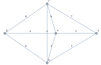
I'm trying to create the following graph in Mathematica

Where do I start? I'm specifically trying to make a graph so that I can use it in TravelingSalesman[g], for g a graph. This is what I have:

g := Graph[{1 \[UndirectedEdge] 2, 1 \[UndirectedEdge] 3, 
   1 \[UndirectedEdge] 5, 1 \[UndirectedEdge] 4, 
   4 \[UndirectedEdge] 5, 4 \[UndirectedEdge] 3, 
   4 \[UndirectedEdge] 2, 3 \[UndirectedEdge] 5, 
   3 \[UndirectedEdge] 2, 2 \[UndirectedEdge] 5}, 
  EdgeWeight -> {4, 5, 6, 3, 4, 5, 6, 7, 2, 7}]

Calling

TravelingSalesman[g]

I get the following result:

Table::iterb: Iterator {Combinatorica`Private`i$828,V[Graph[{1\[UndirectedEdge]2,1\[UndirectedEdge]3,1\[UndirectedEdge]5,1\[UndirectedEdge]4,4\[UndirectedEdge]5,4\[UndirectedEdge]3,4\[UndirectedEdge]2,3\[UndirectedEdge]5,3\[UndirectedEdge]2,2\[UndirectedEdge]5},EdgeWeight->{4,5,6,3,4,5,6,7,2,7}]]} does not have appropriate bounds. >>

Join::heads: Heads Combinatorica`Private`Double and Table at positions 1 and 2 are expected to be the same. >>

Join::heads: Heads Combinatorica`Private`Double and Table at positions 1 and 2 are expected to be the same. >>

Join::heads: Heads Combinatorica`Private`Double and List at positions 1 and 2 are expected to be the same. >>

General::stop: Further output of Join::heads will be suppressed during this calculation. >>

Table::iterb: Iterator {V[Graph[{1\[UndirectedEdge]2,1\[UndirectedEdge]3,1\[UndirectedEdge]5,1\[UndirectedEdge]4,4\[UndirectedEdge]5,4\[UndirectedEdge]3,4\[UndirectedEdge]2,3\[UndirectedEdge]5,3\[UndirectedEdge]2,2\[UndirectedEdge]5},EdgeWeight->{4,5,6,3,4,5,6,7,2,7}]]} does not have appropriate bounds. >>

Table::iterb: Iterator {V[Graph[{1\[UndirectedEdge]2,1\[UndirectedEdge]3,1\[UndirectedEdge]5,1\[UndirectedEdge]4,4\[UndirectedEdge]5,4\[UndirectedEdge]3,4\[UndirectedEdge]2,3\[UndirectedEdge]5,3\[UndirectedEdge]2,2\[UndirectedEdge]5},EdgeWeight->{4,5,6,3,4,5,6,7,2,7}]]} does not have appropriate bounds. >>

General::stop: Further output of Table::iterb will be suppressed during this calculation. >>

Range::range: Range specification in Range[V[Graph[{1\[UndirectedEdge]2,1\[UndirectedEdge]3,1\[UndirectedEdge]5,1\[UndirectedEdge]4,4\[UndirectedEdge]5,4\[UndirectedEdge]3,4\[UndirectedEdge]2,3\[UndirectedEdge]5,3\[UndirectedEdge]2,2\[UndirectedEdge]5},EdgeWeight->{4,5,6,3,4,5,6,7,2,7}]]] does not have appropriate bounds. >>

TravelingSalesman::ham: The graph must contain a Hamiltonian cycle for a traveling salesman tour to be found. >>

Answer 1

Mathematica's graphing features are very powerful, but I find them confusing - there seems to be two separate types of graphing function (not including the deprecated "Combinatorica" system), and not all of the documentation has been written or updated that needs to be. But here's some more ideas for you to play with, to supplement the existing answers.

Some basic data:

data = {{"a" \[UndirectedEdge] "b" -> 3}, 
        {"a" \[UndirectedEdge] "e" -> 5},
        {"a" \[UndirectedEdge] "c" -> 6},
        {"a" \[UndirectedEdge] "d" -> 4}, 
        {"b" \[UndirectedEdge] "c" -> 4}, 
        {"b" \[UndirectedEdge] "e" -> 5}, 
        {"b" \[UndirectedEdge] "d" -> 6}, 
        {"c" \[UndirectedEdge] "e" -> 7}, 
        {"c" \[UndirectedEdge] "d" -> 8}}

from which you can extract the edges and the edge weights:

edges = data[[All, 1, 1]];
edgeweights = data[[All, 1, 2]];

So here's the basic graph:

g = Graph[edges, 
  EdgeWeight -> edgeweights, 
  EdgeLabels -> "EdgeWeight",
  VertexLabels -> "Name", 
  DirectedEdges -> False]

You can use GraphDistance to find the distance between vertices:

GraphDistance[g, #] & /@ VertexList[g]

{{0, 3., 5., 6., 4.}, 
 {3., 0, 5., 4., 6.}, 
 {5., 5., 0, 7., 9.}, 
 {6., 4., 7., 0, 8.}, 
 {4., 6., 9., 8., 0}}

Then you apply a similar process to a list of all the cycles:

cycles = Table[
    {
     Total[GraphDistance[g, First[#], Last[#]] & /@ cycle], 
     cycle
    }, 
  {cycle, FindHamiltonianCycle[g, All]}]

This adds the distances up for each Hamiltonian cycle.

{{29., {"a" <-> "e", "e" <-> "c", "c" <-> "d", "d" <-> "b", "b" <-> "a"}}, 
 {27., {"a" <-> "b", "b" <-> "e", "e" <-> "c", "c" <-> "d", "d" <-> "a"}}, 
 {26., {"a" <-> "d", "d" <-> "c", "c" <-> "b", "b" <-> "e", "e" <-> "a"}}, 
 {30., {"a" <-> "c", "c" <-> "d", "d" <-> "b", "b" <-> "e", "e" <-> "a"}}, 
 {26., {"a" <-> "e", "e" <-> "c", "c" <-> "b", "b" <-> "d", "d" <-> "a"}}, 
 {28., {"a" <-> "c", "c" <-> "e", "e" <-> "b", "b" <-> "d", "d" <-> "a"}}}

Sort this:

sortedCycles = Sort[cycles, First[#1] < First[#2] &];

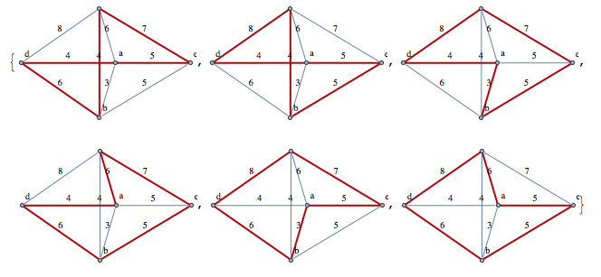
and you can show them using HighlightGraph:

HighlightGraph[g, #, GraphHighlightStyle -> "Thick", 
    ImageSize -> 200] & /@ sortedCycles[[All, 2]]

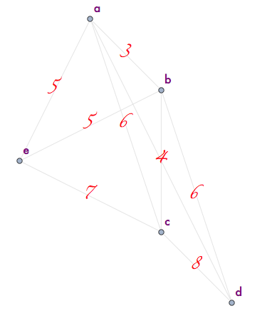
Getting the graphs to look like your original is the next step. Create a layered graph using LayeredGraphPlot, and extract the vertices from it:

vc = VertexCoordinateRules /. 
   Cases[LayeredGraphPlot[AdjacencyMatrix[g]], _Rule, Infinity]

(LayeredGraphPlot is one of the "old" graphing functions, producing graphics and graphics complexes rather than Graph objects.)

Now apply these vertex coordinates to a new graph, defined as before:

h = Graph[edges, 
  EdgeWeight -> edgeweights, 
  EdgeStyle -> LightGray,
  EdgeLabelStyle -> Directive[{FontFamily -> "Zapfino", 16, Red}],
  EdgeLabels -> Flatten[data, 1], 
  VertexLabels -> "Name", 
  VertexLabelStyle -> Directive[{FontFamily -> "Futura", 16, Purple}],
  DirectedEdges -> False, 
  VertexCoordinates -> vc]

which is starting to move close to your original.

I don't know how to create the curved edges. But when I start to play with the fonts and colors, it's an indication that it's time to stop.

Answer 2

You could create weighted adjacency matrix to use as distance matrix in FindShortestTour:

g = Graph[{1 \[UndirectedEdge] 2, 1 \[UndirectedEdge] 3, 
  1 \[UndirectedEdge] 5, 1 \[UndirectedEdge] 4, 
  4 \[UndirectedEdge] 5, 4 \[UndirectedEdge] 3, 
  4 \[UndirectedEdge] 2, 3 \[UndirectedEdge] 5, 
  3 \[UndirectedEdge] 2, 2 \[UndirectedEdge] 5}, 
  EdgeWeight -> {4, 5, 6, 3, 4, 5, 6, 7, 2, 7}, 
  VertexLabels -> Placed["Name", Center],    
  VertexSize -> .3, EdgeLabels -> "EdgeWeight", 
  GraphLayout -> "LayeredDigraphEmbedding", ImagePadding -> 5];

d = ((WeightedAdjacencyMatrix[g] // Normal) /. {0 -> Infinity});

{len, tour} = FindShortestTour[Range[VertexCount[g]], 
     DistanceFunction ->   (d[[#1, #2]] &)]

HighlightGraph[g, UndirectedEdge @@@ Partition[VertexList[g][[tour]], 2, 1, 1], 
 GraphHighlightStyle -> "Thick"]

Answer 3

SetDirectory[NotebookDirectory[]];
img = Import["a.png"];

g = LayeredGraphPlot[{{"a" -> "b", 3}, {"a" -> "e", 5}, {"a" -> "c", 6}, {"a" -> "d", 
     4}, {"b" -> "c", 4}, { "b" -> "e", 5}, {"b" -> "d", 
     6}, {"c" -> "e", 7}, { "c" -> "d", 8}}, 
   PlotStyle -> {Opacity[.5], Gray}, 
   BaseStyle -> {Bold, FontSize -> 24}, VertexLabeling -> True, 
   VertexRenderingFunction -> (Inset[Framed[Style[#2, 22], Background -> White,
      FrameStyle -> Gray], #1, {Center, Top}] &), DirectedEdges -> False, 
      PlotRangePadding -> Automatic,ImageSize -> 450];

Grid[{{img, g}}, Frame -> All]

Answer 4

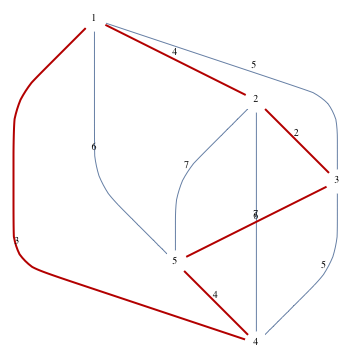
This is a small graph and the unweighted graph has a number of Hamiltonian cycles. I assume the aim is to find the one with minimum cost/weight. This is an approach. I have changed the vertices a,b,c,d,e to 1,2,3,4,5.

g = Graph[{1 \[UndirectedEdge] 2, 2 \[UndirectedEdge] 3, 
   3 \[UndirectedEdge] 4, 4 \[UndirectedEdge] 1, 
   1 \[UndirectedEdge] 3, 3 \[UndirectedEdge] 5, 
   4 \[UndirectedEdge] 5, 2 \[UndirectedEdge] 5, 
   1 \[UndirectedEdge] 5, 2 \[UndirectedEdge] 4}, 
  EdgeWeight -> {3, 4, 7, 4, 6, 7, 2, 5, 5, 6}, 
  VertexLabels -> "Name", EdgeLabels -> "EdgeWeight"];
h = FindHamiltonianCycle[g, All];
norm = Normal@WeightedAdjacencyMatrix[g];
ans = Total /@ (Extract[norm, #] & /@ (# /. 
        a_ \[UndirectedEdge] b_ :> {a, b}) & /@ h);
min = Extract[h, Position[ans, Min[ans]]]
HighlightGraph[g, min, GraphHighlightStyle -> "Thick"]

If I have coded your graph in error I apologise. It would be helpful to code the graph (vertices, edges and edgeweights).