How to plot a matrix with this 3D style in a bar chart?

Question

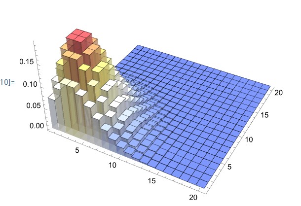
Reading the paper Measuring Wigner functions of quantum states of light in the undergraduate laboratory in arXiv, I found the figure above, whose style is very beautiful. I tried to reproduce it, but I failed. Is there an elegant method to obtain a similar style of bar chart?

code:

alpha = 2;
rho[m_, n_] :=  Exp[-Abs[alpha]^2] alpha^n Conjugate[alpha]^m/Sqrt[n! m!]
matrix = Table[rho[m,n],{m,1,20},{n,1,20}];
MatrixPlot[matrix]

I don't know how to plot a 3d bar chart using a matrix, because my data is created by numerical calculation. I found some example in StackExange, but there the data has n * 5 dimensions.

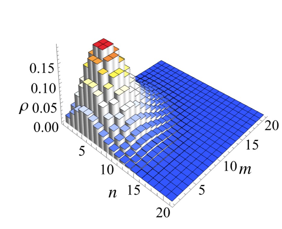
Through trying, I found the following ways to achieve my requirements, thank you all. The effect has not yet been fully reproduced, I will continue to work hard.

revised code version:

alpha=2;
rho[m_,n_]:=Exp[-Abs[alpha]^2] alpha^n Conjugate[alpha]^m/Sqrt[n! m!]
matrix=Table[rho[m,n],{m,1,20},{n,1,20}];
DiscretePlot3D[Abs[matrix[[m,n]]],{m,1,20},{n,1,20},ExtentSize->Full,
ColorFunction->Function[{x,y,z},ColorData["TemperatureMap"]z]],
ColorFunctionScaling->True,BoxRatios->{1, 1, 0.618},Boxed->False]

Answer 1

alpha = 2;
rho[m_, n_] := 
 Exp[-Abs[alpha]^2] alpha^n Conjugate[alpha]^m/Sqrt[n! m!]
matrix = Table[rho[m, n], {m, 1, 21}, {n, 1, 21}];

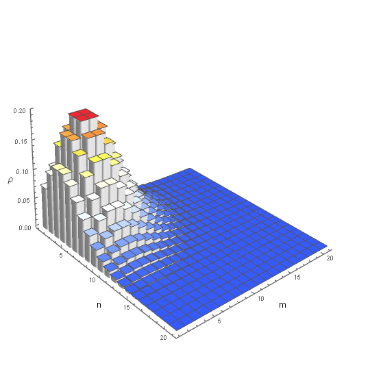
p1 = DiscretePlot3D[Abs[matrix[[m, n]]]
  , {m, 1, 20}, {n, 1, 20}
  , ExtentSize -> Right
  , ExtentMarkers -> None
  , AxesLabel -> (Style[#, Black, 14] & /@ {"n", "m", "\[Rho]"})
  , ExtentElementFunction -> "ProfileCube"
  , PlotStyle -> Opacity[0.9, White]
  , BoxRatios -> {1, 1, 0.618}
  , Boxed -> False
  , SphericalRegion -> True
  , AxesEdge -> {{0, -1}, {1, -1}, {0, -1}}
  , ImagePadding -> {{30, 20}, {30, 20}}
  , ImageSize -> 600
  ];

p2 = ListPlot3D[matrix + 0.001
  , PlotRange -> Full
  , DataRange -> {{1, 21}, {1, 21}}
  , Mesh -> None
  , BoundaryStyle -> {Lighter@Black, AbsoluteThickness[1]}
  , InterpolationOrder -> 0
  , ColorFunction -> 
   Function[{x, y, z}, ColorData["TemperatureMap"][z]]
  , ColorFunctionScaling -> True
  , BoxRatios -> {1, 1, 0.618}
  , Boxed -> False
  , ImageSize -> 600
  ];

Show[p1, p2]

Answer 2

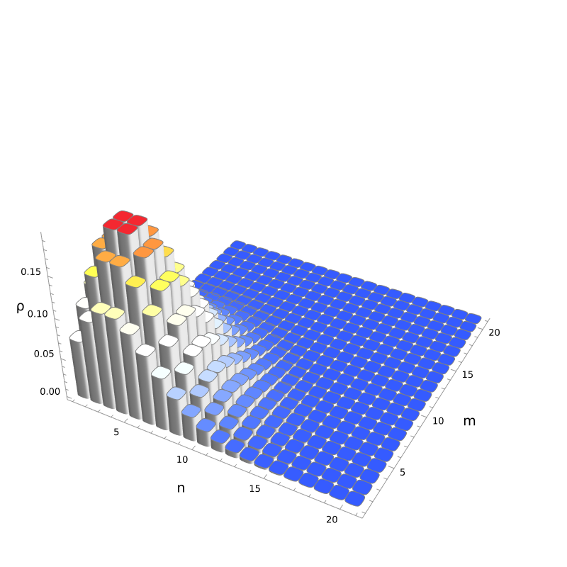
Use the built-in ExtentElementFunction "ProfileCube" to construct two custom functions, one for the caps and the other for sides:

ClearAll[caps, sides]

caps[profile_ : 2] := {EdgeForm[Gray], 
    ChartElementData["ProfileCube", 
     "Profile" -> profile][{#[[1]], #[[2]], {1, 1} #[[3, 2]]}, ##2]} &;

sides[profile_ : 2] :=
   ChartElementData["ProfileCube", "Profile" -> profile][##] /. 
     Rule["SurfaceCaps", _] -> Rule["SurfaceCaps", False] &;

Example:

alpha = 2;

rho[m_, n_] :=  Exp[-Abs[alpha]^2] alpha^n Conjugate[alpha]^m/Sqrt[n! m!]

matrix = Table[rho[m, n], {m, 1, 21}, {n, 1, 21}];

options = Sequence[
   AxesLabel -> (Style[#, Black, 14] & /@ {"n", "m", "ρ"}),
   ExtentSize -> Right, 
   ExtentMarkers -> None,
   AxesEdge -> {{0, -1}, {1, -1}, {0, -1}},
   BoxRatios -> {1, 1, 0.618},
   Boxed -> False, 
   SphericalRegion -> True,
   ImagePadding -> {{30, 20}, {30, 20}}, 
   ImageSize -> 600];

pa = DiscretePlot3D[Abs[matrix[[m, n]]], 
   {m, 1, 20}, {n, 1, 20},
   ColorFunction -> "TemperatureMap",
   ExtentElementFunction -> caps[],
   Evaluate @ options];

pb = DiscretePlot3D[Abs[matrix[[m, n]]], {m, 1, 20}, {n, 1, 20}, 
   ExtentElementFunction -> sides[], 
   FillingStyle -> White, 
   Evaluate @ options];

Post-process pa to fix the colors:

Show[pa /. BSplineSurface[a_, b___] :> 
    {ColorData["TemperatureMap"][
        Rescale[a[[1, 1, -1]], MinMax @ Abs @ matrix]], 
      BSplineSurface[a, b]},
    pb]