Galactic rotation speed

Question

Rotation speed vc[R] in reduced units for M33 looks like

0.342331 Sqrt[R^2/(0.728117 + R^2)^0.87955]

Knowing e=0.995, I am trying to get the density Rho[m]from the equation

vc[R]^2 == Integrate[(4 Pi Sqrt[1 - e^2] m^2  Rho[m])/  Sqrt[-e^2 m^2 + R^2], {m, 0, R}]

This equation comes from Galactic Dynamics Binney Tremaine 2008. (2.132)

Using trial and error, I obtain a "good" solution for Rho[m], but it is very time expensive.

Does anybody knows how to solve this equation to get Rho[m]?

Thanks in advance.

Answer 1

Here my third answer which solves case R==25 .

This approach uses an interpolation-function (instead of wavelets or FEM) to describe the unknown function rho[R] and evaluates the integrations using Gauss quadratur.

e = 0.995;
v[R_] := 0.342331 Sqrt[R^2/(0.728117 + R^2)^0.87955] ;
Rmin = 0; Rmax = 25;
ni = 25 ; 

Get["NumericalDifferentialEquationAnalysis`"];  

(* grid R *)
riGrid[n_] := 
Block[{dt, \[CapitalDelta]t0, \[CapitalDelta]t1, zw, sol}, 
dt = Map[ \[CapitalDelta]t0 + (\[CapitalDelta]t1 - \
\[CapitalDelta]t0) (#/Rmax)^2 &, Subdivide[0, Rmax, n]];
zw = Accumulate[dt] ;
sol = Solve[{zw[[1]] == 0,zw[[-1]] == Rmax}, {\[CapitalDelta]t0,\[CapitalDelta]t1}][[1]];
zw /. sol  // N]

ri=riGrid[ni]; (* problem adapted grid *)
\[Rho]i = Array[\[Rho], Length[ri]];
swGauss = 
 GaussianQuadratureWeights[ 15, 0, e] ;(*Stützstellen&Gewichte*)

 
zwv = Function[{RR}, Evaluate[  v[RR] ^2/(4 Pi RR^2 ) ]];

JJ = Sum[ (zwv[R]   - 
      Sqrt[1 - e^2]/
       e^3 Total@
        Map[#[[2]] #[[1]]^2 /
           Sqrt[1 - #[[1]]^2] Interpolation[
             Transpose[{Rationalize[ri], \[Rho]i}]][#[[1]]  R/e ] & , 
         swGauss] )^2, {R, ri}];
mini00 = NMinimize[{JJ }, \[Rho]i]; // AbsoluteTiming
ListPlot[Rest@Transpose[{ri, \[Rho]i} /. mini00[[2]]]]

Answer 2

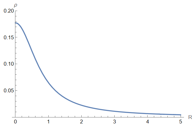
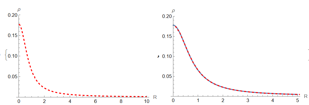
We can solve this problem using colocation method with Euler wavelets ang Gauss quadrature rule. First we define interval $0\le R\le Rmax$ and map interval $(0,R)$, on R/2 (1+z) with $-1\le z \le 1$ in integrand, then the Volterra integral equation becomes Fredholm integral equation. Before code please call

Get["NumericalDifferentialEquationAnalysis`"];

Code

e = 0.995;
v[R_] := 0.342331 Sqrt[R^2/(0.728117 + R^2)^0.87955];
Rmin = 0; Rmax = 5;
UE[m_, t_] := EulerE[m, t];
psi[k_, n_, m_, t_] := 
  Piecewise[{{2^(k/2)  UE[m, 2^k t - 2 n + 1], (n - 1)/2^(k - 1) <= 
      t < n/2^(k - 1)}, {0, True}}];
PsiE[k_, M_, t_] := 
 Flatten[Table[psi[k, n, m, t], {n, 1, 2^(k - 1)}, {m, 0, M - 1}]]
k0 = 4; M0 = 7; With[{k = k0, M = M0}, 
 nn = Length[Flatten[Table[1, {n, 1, 2^(k - 1)}, {m, 0, M - 1}]]]];
dx = 1/(nn); xl = Table[l*dx, {l, 0, nn}]; M = nn; np = nn; g = 
 GaussianQuadratureWeights[np, -1, 1];
ugrid = g[[All, 1]]; weights = g[[All, 2]]; xcol = 
 Table[(xl[[l - 1]] + xl[[l]])/2, {l, 2, nn + 1}]; Psijk = 
 With[{k = k0, M = M0}, PsiE[k, M, t1]];
Psi[y_] := Psijk /. t1 -> y;
A = Array[a, nn]; Rho[y_] := A . Psi[y];
eqs = Table[
   v[Rmax x]^2 == 
    0.31376632053307746 (Rmax x)^2/
      2 Sum[( (1 + z)^2 Rho[ 1/2 x (1 + z)] weights[[i]])/Sqrt[
       1 - 0.24750625 (1 + z)^2] /. z -> ugrid[[i]], {i, np}], {x, 
    xcol}];

{vec, mat} = CoefficientArrays[eqs, A]

sol = LinearSolve[mat // N, -vec];

rul = Table[A[[i]] -> sol[[i]], {i, nn}]; p=Plot[
 Rho[x/Rmax] /. rul, {x, 0, Rmax}, PlotRange -> {0, .2}, AxesLabel -> {"R", "\[Rho]"}]

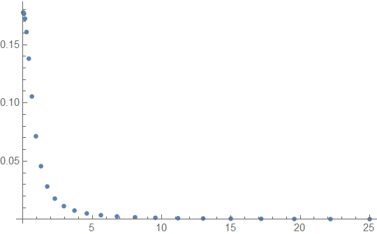
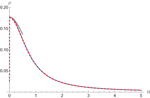
Update 1. We can compare this solution (solid line) with Ulrich solution at Rmax=5 (red dashed line) as follows

    e = 0.995;
v[R_] := 0.342331 Sqrt[R^2/(0.728117 + R^2)^0.87955];
Rmin = 0; Rmax = 5;
ni = 50;
ri = Subdivide[Rmin, Rmax, ni];

f[G_] := 
  Block[{R, m, zw = Simplify[v[R] v'[R]/(2 \[Pi] R)]}, 
   Interpolation[
    Table[{R, ( 
       Sqrt[1 - e^2]/e^3 NIntegrate[( s^2 G[s R/e])/(-s^2 + 1)^(
          3/2), {s, 0, e}, Method -> "LocalAdaptive"] + zw )}, {R, 
      ri}]]];

solf = NestList[f, .18/(1 + #^2) &, 20]; p1 = 
 Plot[solf[[-1]][R], {R, Rmin, Rmax}, PlotStyle -> {Dashed, Red}]
   
    Show[p,p1] 

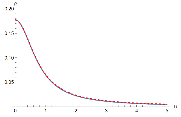
We see a small discrepancy that disappears as the number of iterations increases.

Update 2. We can use also power series as Stephen proposed. Using NMinimize we can simplifier this method as follows (m->R/e s)

int = 
 Table[Integrate[( s^2 s^i)/Sqrt[- s^2 + 1], s], {i, 0, 10}];

int0 = N[int /. s -> 10^-16, 30];

int1 = int /. s -> e;

A = Table[(R/e)^i, {i, 0, 10}]; B = Array[b, Length[A]];

dint = int1 - int0; r = Range[0, 1, 1/10];  
eq = Table[-v[R]^2 + 
    4 Pi Sqrt[1 - e^2] R^2/e^3 Sum[
      A[[i]] B[[i]] dint[[i]], {i, Length[A]}], {R, r}];

sol1 = NMinimize[eq . eq, B];

p2 = Plot[A . B /. sol1[[2]], {R, 0, 1}, PlotStyle -> {Red, Dashed}];

Visualization together with wavelets solution

Show[p,p2]

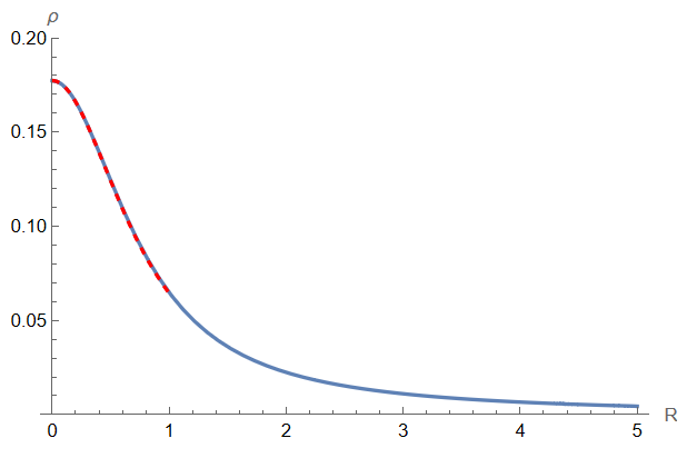
We see nice agreement for power series solution and wavelets solution. Note that we can extend power series up to R=5 using this code

e = 0.995;
v[R_] := 0.342331 Sqrt[R^2/(0.728117 + R^2)^0.87955];
Rmin = 0; Rmax = 5;

int = Table[Integrate[(s^2 s^i)/Sqrt[-s^2 + 1], s], {i, 0, 10}];

int0 = N[int /. s -> 10^-16, 30];

int1 = int /. s -> e;

A = Table[(R/e)^i, {i, 0, 10}]; B = Array[b, Length[A]];

dint = int1 - int0;
Do[rr[i] = Subdivide[i, i + 1, Length[A]];
  eqs[i] = 
   Table[-v[R]^2 + 
     4 Pi Sqrt[1 - e^2] R^2/e^3 Sum[
       A[[i]] B[[i]] dint[[i]], {i, Length[A]}], {R, rr[i]}];
  sol[i] = NMinimize[eqs[i] . eqs[i], B]; 
  pp[i] = Plot[A . B /. sol[i][[2]], {R, i, i + 1}, 
    PlotStyle -> {Red, Dashed}, PlotRange -> All];, {i, 0, 4}];

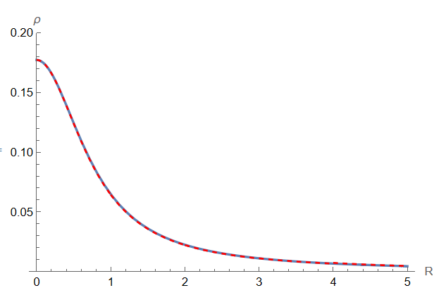
Finally we compare power series solution and wavelets solutions in one plot

Show[p,Table[pp[i], {i, 0, 4}]] 

Update 3. To compute solution up to R=10 we need to improve wavelets numerical algorithm using NIntegrate instead of the Gauss quadrature rule. So we have

e = 0.995; lambda = 4 Sqrt[1 - e^2] \[Pi] /e^3;
v[R_] := 0.342331 Sqrt[R^2/(0.728117 + R^2)^0.87955];
UE[m_, t_] := EulerE[m, t];
psi[k_, n_, m_, t_] := 
  Piecewise[{{2^(k/2) UE[m, 2^k t - 2 n + 1], (n - 1)/2^(k - 1) <= t <=
       n/2^(k - 1)}, {0, True}}];
PsiE[k_, M_, t_] := 
 Flatten[Table[psi[k, n, m, t], {n, 1, 2^(k - 1)}, {m, 0, M - 1}]]
k0 = 4; M0 = 7; With[{k = k0, M = M0}, 
 nn = Length[Flatten[Table[1, {n, 1, 2^(k - 1)}, {m, 0, M - 1}]]]];
dx = 1/(nn); xl = Table[l*dx, {l, 0, nn}]; xcol = 
 Table[(xl[[l - 1]] + xl[[l]])/2, {l, 2, nn + 1}]; Psijk = 
 With[{k = k0, M = M0}, PsiE[k, M, t1]];
Psi[y_] := Psijk /. t1 -> y;
A = Array[a, nn]; Rho[y_] := A . Psi[y];
int[x_] := 
  NIntegrate[ z^2 Psi[( x z)/e]/Sqrt[1 - z^2], {z, 0, e}, 
   Method -> "LocalAdaptive", AccuracyGoal -> 5];
eq[Rmin_, Rmax_] := 
  Table[(v[Rmin + (Rmax - Rmin) x]/(Rmin + (Rmax - Rmin) x))^2 == 
    lambda A . int[x], {x, xcol}];

Numerical solution

sol10 = NSolve[eq[0, 10], A];

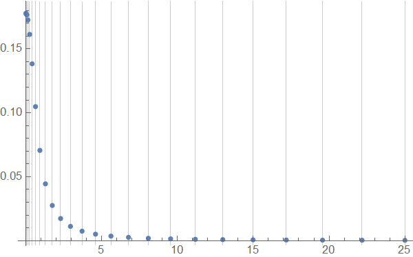
Visualization together with p and separately

{p10 = Plot[Rho[x/10] /. sol10[[1]], {x, 0, 10}, PlotRange -> {0, .2}, 
   AxesLabel -> {"R", "\[Rho]"}, PlotStyle -> {Red, Dashed}], Show[p,p10]}
    

Answer 3

Here is a series expansion solution based on the idea that I mentioned in an earlier comment. Within the range of validity of the series expansion it leads to a result that is numerically very similar to the result obtained by Alex Trounev.

Definitions given in the original question.

vc[R_] = 0.342331 Sqrt[R^2/(0.728117 + R^2)^0.87955]

eqn[R_, e_] = 
 vc[R]^2 == 
  Integrate[(4 Pi Sqrt[1 - e^2] m^2 Rho[m])/Sqrt[-e^2 m^2 + R^2], {m, 0, R}]

The solution strategy is to use the series expansion of the equation about R = 0 to compute the derivatives of Rho[m] at m = 0.

Check the first few terms of this series for e = 0.995.

eqnSeries = Series[eqn[R, 0.995], {R, 0, 2}] // PowerExpand;
SolveAlways[eqnSeries, R]
(* {{Rho[0] -> 0.177325}} *)

eqnSeries = Series[eqn[R, 0.995], {R, 0, 3}] // PowerExpand;
SolveAlways[eqnSeries, R]
(* {{Rho[0] -> 0.177325, Derivative[1][Rho][0] -> 0.}} *)

eqnSeries = Series[eqn[R, 0.995], {R, 0, 4}] // PowerExpand;
SolveAlways[eqnSeries, R]
(* {{Rho[0] -> 0.177325, Derivative[1][Rho][0] -> 0., (Rho^\[Prime]\[Prime])[0] -> -0.593919}} *)

Switch to a fully algebraic solution. Save the variable values in a list of rules for later use.

vals = {a -> 0.342331, b -> 0.728117, c -> 0.87955, e -> 0.995};

Fully algebraic version of the definitions given in the question. Transform the integral using m = R s so that 0 < m < R is transformed to 0 < s < 1.

vc[R_, {a_, b_, c_}] = a Sqrt[R^2/(b + R^2)^c]

eqn[R_, {a_, b_, c_}, e_] = 
 vc[R, {a, b, c}]^2 == 
  R^2 Integrate[(4 Pi Sqrt[1 - e^2] s^2 Rho[R s])/Sqrt[-e^2 s^2 + 1], {s, 0, 1}]

Coefficient of R^p on the left hand side of the equation.

lhs[p_] = SeriesCoefficient[eqn[R, {a, b, c}, e][[1]], {R, 0, p}]

(* piecewise expression with all odd-p coefficients being zero *)

Series expand Rho[x] about x = 0.

Sum[(x^p/p!)*Derivative[p][Rho][0], {p, 0, Infinity}]

The p-th term of the series on the right hand side of the equation.

rhs[p_] = 
 Assuming[{0 < e <= 1, p >= 0, p \[Element] Integers}, 
  (eqn[R, {a, b, c}, e][[2]] /. {Rho[R s] -> (R s)^p/p! Derivative[p][Rho][0]})]

(* expression with a hypergeometric function in it *)

Equate corresponding powers on the left and right hand sides of the equation, and solve for the corresponding derivative of Rho[x] at x = 0.

eqnSeries = Simplify[lhs[p + 2] R^(p + 2)] == rhs[p];
soln = Solve[eqnSeries, Derivative[p][Rho][0]][[1]] // 
  Simplify[#, Assumptions -> {a > 0, 0 < b < 1, 0 < c < 1, p \[Element] Integers, p >= 0}] &

(* piecewise expression for Derivative[p][Rho][0] with all odd-p derivatives being zero *)

Substitute in the numerical values of the variables.

solnN = soln /. vals // Simplify[#, Assumptions -> {p \[Element] Integers, p >= 0}] &

Compute a table of the first few terms of the series expansion Rho[x] about x = 0.

Table[{p, R^p Derivative[p][Rho][0]/p!} /. solnN /. {R -> 0.5}, {p, 0, 10}] // Grid

(* table showing nice series convergence, at least for this value of R *)

Here is a rough-and-ready routine (0 < R < 0.82 or thereabouts) for numerically summing the series.

sumSeries[R_, error_ : 10^(-6)] :=
  Module[{term = 1, sum = 0, q = 0, qstep = 2, coefft},
   coefft = Derivative[p][Rho][0] /. solnN;
   While[Abs[term] > error,
    term = R^p coefft/p! /. p -> q;
    sum += term;
    q += qstep];
   sum
   ];

Plot Rho[R].

Plot[sumSeries[R], {R, 0, 0.82}, PlotRange -> {Automatic, {0, 0.2}}, 
 Frame -> True, FrameLabel -> {"R", "Rho[R]"}]

This numerical result is very similar to the one computed by Alex Trounev. However I find that my series expansion diverges for R > 0.82 or thereabouts.

Answer 4

Here I 'll show an iterative solution.

First the integralequation is differentiated D[....,R] . This finally gives

rho[R] == (v[R] v'[R])/(2 Pi R) + Integrate[rho[m] m^2 Sqrt[1 - e^2]/Sqrt[R^2 - e^2 m^2]^3 , {m, 0, R} ]

This integralequation is solved numerically (using NIntegrate , Interpolation and NestList)

e = 0.995;
v[R_] := 0.342331 Sqrt[R^2/(0.728117 + R^2)^0.87955] //Rationalize[#, 0] &;
Rmin = 0; Rmax = 10;
ni =  25;  
ri = Subdivide[0, Rmax, ni];

gfip[G_] := Block[{ R, m, zw = Simplify[(v[R] v'[R])/(2 Pi R)]},
Interpolation[Table[{R, 
 zw + NIntegrate[G[m] m^2  Sqrt[1 - e^2]/Sqrt[R^2 - e^2 m^2]^3 , {m, 0, R}  , 
   Method ->  "LocalAdaptive"  ] }, {R, ri}]   ]]
solf=solf = NestList[gfip, 0 &, 10]; 

Plot[ solf[[-1]] [R] , {R, 0, Rmax}, PlotRange -> All,AxesLabel -> {"R", "rho[R]"}]

Answer 5

modified: Case Rmax==25

Inspired by the interesting discussion with Alex I found a direct approach, using a simple polygonal ansatz( borrowed from FEM). It solves the original integralequation, transformed via m->s R/e.

e = 0.995;
v[R_] := 0.342331 Sqrt[R^2/(0.728117 + R^2)^0.87955] ;
Rmin = 0; Rmax = 25;
ni = 25 ; 

Needs["NDSolve`FEM`"]

riGrid[n_] := 
Block[{dt, \[CapitalDelta]t0, \[CapitalDelta]t1, zw, sol}, 
dt = Map[ \[CapitalDelta]t0 + (\[CapitalDelta]t1 - \
\[CapitalDelta]t0) (#/Rmax)^2 &, Subdivide[0, Rmax, n]];
zw = Accumulate[dt] ;
sol = Solve[{zw[[1]] == 0,zw[[-1]] == Rmax}, {\[CapitalDelta]t0,\[CapitalDelta]t1}][[1]];
zw /. sol  // N]

ri=riGrid[ni]; (* problem adapted grid *)
\[Rho]i = Table[\[Rho][k], {k, 1, Length[ri]}];

netz = ToElementMesh[Map[{#} &, ri]]
\[Phi]i =Map[ElementMeshInterpolation[netz, #] &,IdentityMatrix[Length[ri]]];

Plot[Evaluate[Through[\[Phi]i[R]]], {R, 0, Rmax}]
[![enter image description here][1]][1]

int[R_?NumericQ] := 
Block[{zwv = Function[{RR}, Evaluate[  v[RR] ^2/(4 Pi RR^2 ) ]]},
zwv[R] -Sqrt[1 - e^2]/e^3 NIntegrate[s^2 /Sqrt[1 - s^2] Through[\[Phi]i[s R/e]], {s, 0, e}, Method -> {"FiniteElement", "LocalAdaptive"}[[1]]] . \[Rho]i]

zwint = Table[int[R], {R, ri}] /. 0. -> 0 // Quiet;
mini0 = NMinimize[zwint . zwint, \[Rho]i ]
ListPlot[Rest@Transpose[{ri, \[Rho]i} /. mini0[[2]]],GridLines->{ri,None}]

The solution agrees quite well with solutions presented by Alex.

Answer 6

Here's a solution based on discretization of the integral using the trapezoid rule: yeah it's simple and naive, but it works!

As shown in other answers, the precision for small $R$ is a bit hard to raise. In this answer, the issue is resolved with graded mesh, which is part of the built-in FEM functionality.

In the following code I've also included a solasymp which is essentially a simplification of Stephen Luttrell's method for small $R$.

e = 0.995;
vc[R_] = 0.342331  Sqrt[R^2/(0.728117 + R^2)^0.87955];

domain = {0, 5}; points = 1000;

<< NDSolve`FEM`
grid = ToGradedMesh[
     Line[List /@ domain], <|"Alignment" -> "Left", "ElementCount" -> points, 
      "GradingRatio" -> 1.01|>, MeshOrder -> 1]["Coordinates"] // Flatten;

Clear@int;
int[expr_, {var_, 0, r_?NumericQ}] := 
 With[{pos = Ordering[Abs[grid - r], 1][[1]]}, 
  trap[Function @@ {var, expr}, grid[[;; pos]]]]

trap[f_, grid_] := 
  With[{dlst = Differences@grid}, (Total[dlst (f /@ Most@grid + f /@ Rest@grid)])/2];

expr = (4 π Sqrt[1 - e^2] m^2 Rho[m])/Sqrt[-e^2 m^2 + R^2];
eq = vc[R]^2 == int[expr, {m, 0, R}];
ae = Table[eq, {R, Rest@grid}]; // AbsoluteTiming
(* {4.3569, Null} *)
    
solasymp[R_] = 
 Rho[R] /. First@
   Simplify[Solve[vc[R]^2 == AsymptoticIntegrate[expr, {m, 0, R}, R -> 0], Rho[R]], 
    R > 0]
(* 0.134143/(0.728117 + R^2)^0.87955 *)
    
sollst = LinearSolve[#2, -#1] & @@ 
    CoefficientArrays[ae, Rho /@ Rest@grid]; // AbsoluteTiming

Show[p, ListLinePlot[{grid // Rest, sollst}\[Transpose], PlotRange -> All, 
  PlotStyle -> {Red, Dashed}], Plot[solasymp[x], {x, 0, 0.5}, PlotStyle -> Gray]]
(* {5.58611, Null} *)

Definition of p is the same as that in Alex's answer. We can see the numeric error for very small $R$ is a bit obvious, but given that the influenced domain is quite narrow, we can simply ignore it. Alternatively, we may turn to the asymptotic solution solasymp to supplement the function value for very small $R$.