Solving a one-dimensional free-boundary problem with a singular boundary condition

Question

Addendum (orginial question below). Thank you for the responses! After thinking some more about this problem, and thanks to @bbgodfreys helpful comment, I realised that the problem as posted below is incomplete. What I need instead is to find $R$ and $f$ such that

1. $f(R) = g(\lambda R)$,
2. $f'(R) = g'(\lambda R)$,
3. $\lim_{r \to 0} \frac{r f'(r)}{f(r)} = -\gamma$, and

$f$ also satisfies the ODE below. This leads to two questions.

Q1. Which two conditions I should pass to NDSolve, and which one should be the focus of the FindRoot operation? Further, what is the correct way to pass condition 3 to NDSolve?

Q2. In either case, the small-$r$ limit and corresponding singularity of $f$ in condition 3 makes life difficult - what is the best way to deal with this?

Perhaps Q1 is not so critical - Q2 seems to me to be the bottleneck. My current attempt, using the methods in the answers below, is to pass conditions 1 and 2 to NDSolve, and use FindRoot for condition 3. I have however been unsuccessul thus far. To wit, if I set $r = 0$ as the left boundary of NDSolve, I first of all get the expected warning

NDSolveValue::ndsz: At r == 1.2839295947759316`*^-19, step size is effectively zero; singularity or stiff system suspected.

This sets a lower bound on $r$ for FindRoot, since I assume from the warning above that I am not to trust the solution for $r < 10^{-19}$. I hence have to make an ad hoc choice for FindRoot for condition 3, for example,

trig = R/.FindRoot[
  -\[Gamma] - (r Derivative[1][solver[R]][r])/solver[R][r] /. CONS /. 
   r -> 10^-15,
  {R, (1/100/1000)/5}
  ][[1]]

(* 4.28145*10^-15 *)

I am unconvinced by FindRoot's solution, since (i) it seems to depend on my ad hoc choice for "$r \to 0$", and (ii) doesn't seem to perform well anyway:

sol = solver[trig]

-\[Gamma] - (r Derivative[1][sol][r])/sol[r] /. CONS /. r -> 10^-15
(* 0.0230768 *)

I'm aware that this addendum significantly alters the question - my apologies! Would be grateful for any suggestions on how to proceed from here. Thanks again for your help thus far.

---

Original question. I have the following ODE for $f(r)$:

pdef = 2 (\[Beta] f[r] + 
r (-\[Mu] + \[Rho]) Derivative[1][f][
      r] + ((-1)^(\[Gamma]/(-1 + \[Gamma])) r^((
     2 \[Gamma])/(-1 + \[Gamma])) (-1 + \[Gamma]) \
\[Zeta]^(-(\[Gamma]/(-1 + \[Gamma]))) \[Rho]^(\[Gamma]/(-1 + \
\[Gamma]))
      Derivative[1][f][r]^(\[Gamma]/(-1 + \[Gamma])))/\[Gamma]) == 
 r^2 \[Sigma]^2 (f^\[Prime]\[Prime])[r]

I am looking for an $R > 0$ such that for the following known function $g$,

g[r_] := (2^(1 - \[Gamma]) (1/
  r)^\[Gamma] \[Eta]^\[Gamma] \[Rho]^-\[Gamma] ((-2 \[Beta] + \
\[Gamma] (-2 \[Mu] + 
      2 \[Rho] + (1 + \[Gamma]) \[Sigma]^2))/(-1 + \[Gamma]))^(-1 + \
\[Gamma]))/\[Gamma]

we have $f(R) = g(\lambda R)$, and $f'(R) = g'(\lambda R)$ for $\lambda$ a constant. Further, for $r < R$, we must have $f(r) > g(r)$, as well as $\lim_{r \to\ 0} f(r) = \infty$

Since I do not know $R$, my idea is to wrap NDSolve in FindRoot as follows. First, for some guess $R$, define

solver[R_?NumericQ] := NDSolveValue[{
   pdef /. CONS,
   DirichletCondition[f[r] == g[\[Lambda] r] /. CONS, r == R]
   },
  f,
  {r, R/10, R}
  ]

where

CONS = {\[Rho] -> 0.02, 
  J -> 5, \[Gamma] -> 0.5, \[Mu] -> 0.03, \[Sigma] -> 0.2, \[Zeta] -> 
   0.5, \[Beta] -> 0.012, k -> 10, \[Eta] -> 0.8, \[Lambda] -> 1.03}

is a set of constants. Then use FindRoot to ensure that the condition on the derivative is specified:

FindRoot[
  Derivative[1][solver[R]][R] - D[g[\[Lambda] R], R] /. CONS,
  {R, 1/100000}
  ]

However, I run into trouble with my function solver, which gives me the error message

DiscretizePDE::femdpop: The FEMLoadElements operator failed.

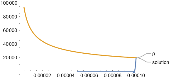
A plot shows that the solution, instead of "shooting" up and above the orange curve, collapses to the $r$-axis.

What is wrong with my NDSolve setup? I would be grateful for any suggestions on how to improve my approach or attack the problem with an alternative method.

PS. I have resorted to the above since I simply could not understand how to implement NeumannValue for this problem. I was also unsuccessful in implementing Method -> "Shooting" with the smooth fit conditions: the solution "collapsed" just as above, leading me to believe that the derivative condition was simply being ignored when shooting.

Answer 1

The question's ode with the given constants, rationalized, is

pdfc = 2 ((3 f[r])/250 + 25/(r^2 f'[r]) - 1/100 r f'[r]) == 1/25 r^2 f''[r]

and the function g is 200/Sqrt[r]. Answering the question is difficult, because the ode has an essential singularity at r = 0, and Limit[r f'[r]/f[r], r->0] can have multiple values.

Approximate symbolic solution of pdfc

Some insight can be gained, however, by obtaining an approximate solution to the ODE, obtained by dropping the term 25/(r^2 f'[r]).

sa = DSolveValue[2 ((3 f[r])/250 - 1/100 r f'[r]) == 1/25 r^2 f''[r], f[r], r]
(* r^(1/2 (1/2 - Sqrt[53/5]/2)) C[1] + r^(1/2 (1/2 + Sqrt[53/5]/2)) C[2] *)

The two exponents have numerical values {-0.563941, 1.06394}. If, then, f[r] is set equal to the first exponential, it is easy to show that the term 25/(r^2 f'[r]) indeed can be ignored for very small r. The same is not true of the second exponential, which should be dropped (e.g., C[2] = 0) from the approximate solution. Consequently, this solution satisfies the limit,

Limit[r f'[r]/f[r], r->0] = 1/4 (1 - Sqrt[53/5])

Interesting, an exact solution also exists, c/Sqrt[r], with {c -> -50 Sqrt[10], c -> 50 Sqrt[10]}.

Simplify[pdfc /. f -> Function[{r}, -50 Sqrt[10]/Sqrt[r]]]
(* True *)

and similarly for the second value of c. As will become apparent below, this solution is not of much value. For completeness, this solution has the small r limit,

Limit[r f'[r]/f[r], r->0] = -1/2

There may be other symbolic solutions, but I have been unable to find any.

Numerical solutions

Obtaining numerical solutions may seem straightforward: With initial conditions, {f[rm] == g[1.03 rm], f'[rm] == g'[1.03 rm]}, integrate toward r = 0. However, integrating toward an essential singularity invites numerical errors. So, I first integrated to a very small value of r0 = 10^-30 and then integrated back again to rm to ascertain whether the same values of `{f[rm], f'[rm]} resulted. It turned out that very high precision was required. For instance,

r0 = 10^-30; rm = 1; wp = 150;
s1 = NDSolveValue[{pdfc, f[rm] == 200/Sqrt[103/100 rm], 
    f'[rm] == -100/Sqrt[103/100 rm]^3}, {f[r], f[r0], f'[r0]}, {r, r0, rm}, 
    WorkingPrecision -> wp, Method -> "StiffnessSwitching", 
    InterpolationOrder -> All];
s2 = NDSolveValue[{pdfc, f[r0] == SetPrecision[s1[[2]], wp], 
    f'[r0] == SetPrecision[s1[[3]], wp]}, {f[r], f[rm], f'[rm]}, {r, r0, rm}, 
    WorkingPrecision -> wp, Method -> "StiffnessSwitching", 
    InterpolationOrder -> All];

A measure of the accuracy of the calculation is

{s2[[2]]/g[103/100 rm]) - 1, s2[[3]]/g'[103/100 rm] - 1} // N
(* {-6.2683*10^-29, 1.27023*10^-28} *)

(Smaller values of wp often perform much less well.) The curves themselves are shown by

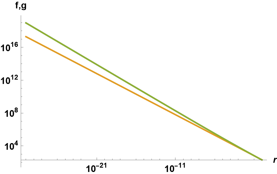
LogLogPlot[{First[s1], g[r], First[s2]}, {r, r0, rm}, 
    AxesLabel -> {r, "f,g"}, LabelStyle -> {12, Bold, Black}]

where the blue and green curves (superimposed) are the inward and outward numerical integrations, and the orange curve is g[r]. More informative is a plot of r f'[r]/f[r].

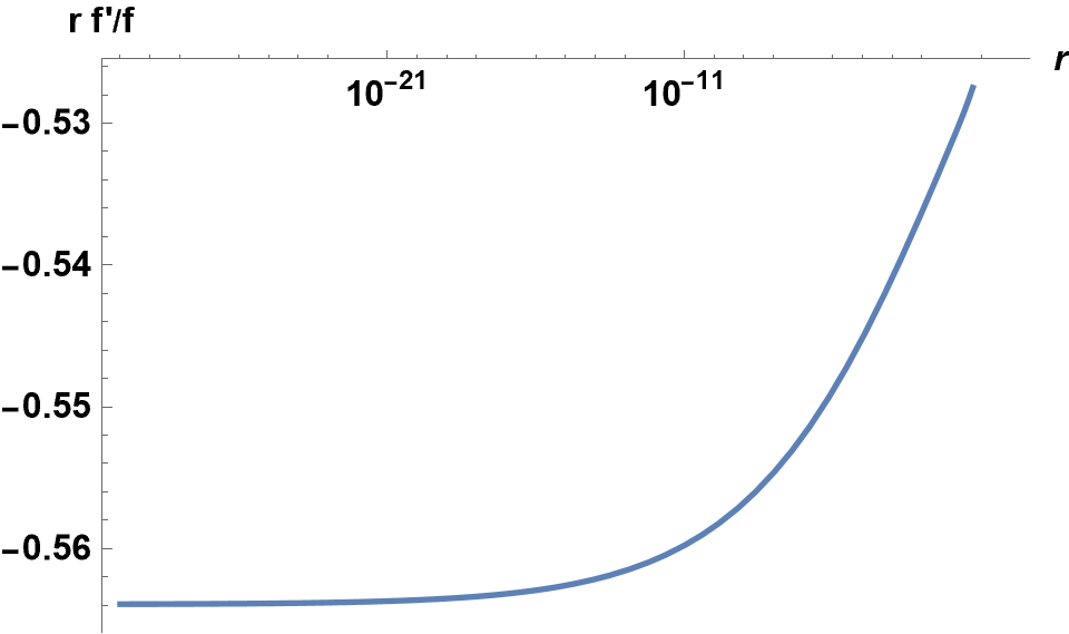
LogLinearPlot[Evaluate[r D[s2[[1]], r]/s2[[1]]], {r, r0, rm}, 
    AxesLabel -> {r, "r f'/f"}, LabelStyle -> {12, Bold, Black}]

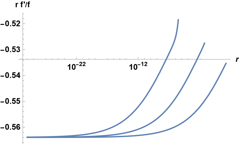
which converges to -0.564 for very small r, as might be expected from the symbolic analysis above. Note that the numerical calculation takes several minutes on my pc. Thus, if this is accepted as the desired r = 0 limit, then rm = 1 satisfies the question. In fact, every value of rm I have tried does so, and in each case Limit[r f'[r]/f[r], r->0] converges to the same value. Curves for rm = {10^-5, 1, 10^5} are

In no case did r f'[r]/f[r] converge to -1/2.

Answer 2

I'm more accustomed to working in a slightly different format, but this should be equivalent to what you're doing. Define functions to build the pdes and g:

pdef[\[Beta]_, \[Gamma]_, \[Sigma]_, \[Mu]_, \[Rho]_, \[Zeta]_] := 
  2 \[Beta] f[r] + 
    2 r (-\[Mu] + \[Rho]) f'[
      r] + (2 (-1)^(\[Gamma]/(-1 + \[Gamma])) r^((2 \[Gamma])/(-1 + \
\[Gamma])) (-1 + \[Gamma]) \[Zeta]^(-(\[Gamma]/(-1 + \[Gamma]))) \
\[Rho]^(\[Gamma]/(-1 + \[Gamma])) f'[
         r]^(\[Gamma]/(-1 + \[Gamma])))/\[Gamma] - 
    r^2 \[Sigma]^2 f''[r] == 0;

g[\[Beta]_, \[Gamma]_, \[Mu]_, \[Eta]_, \[Rho]_, \[Sigma]_, \
\[Lambda]_][
   r_] := (2^(1 - \[Gamma]) (1/
        r)^\[Gamma] \[Eta]^\[Gamma] \[Rho]^-\[Gamma] ((-2 \[Beta] + \
\[Gamma] (-2 \[Mu] + 
             2 \[Rho] + (1 + \[Gamma]) \[Sigma]^2))/(-1 + \
\[Gamma]))^(-1 + \[Gamma]))/\[Gamma];

The solver with most of the constants plugged in. (You don't seem to use J or k for anything as far as I can tell.)

solver[rSol_?NumericQ] := 
  NDSolve[{pdef[0.012, 1/2, 0.2, 0.03, 0.02, 1/2], 
    f[rSol] == g[0.012, 1/2, 0.03, 0.8, 0.02, 0.2, 1.03][rSol], 
    Derivative[1][f][rSol] == 
     Derivative[1][g[0.012, 1/2, 0.03, 0.8, 0.02, 0.2, 1.03]][rSol]}, 
   f, {r, rSol/10, rSol}];

The main difference is that I removed the Dirichlet code and just used a simple f[rSol] = g[..][rSol] and the corresponding derivatives directly, using the conditions you wrote in the text.

FindRoot complained about the solution being non-numeric, so I created an auxillary function to keep it happy:

rsf[rs_?NumericQ] := 
  Derivative[1][f][rs] /. Flatten@solver[rs];

I changed the constant to a value different from yours, to verify that it did indeed search for the root:

FindRoot[
 rsf[rSol] - 
  Derivative[1][g[0.012, 1/2, 0.03, 0.8, 0.02, 0.2, 1.03]][
   rSol], {rSol, .0002(*1/100000*)}]

Out[39]= {rSol -> 0.00001}

I reran once last time to generate plots and verify other conditions. The output was of the form {f->InterpolatingFunction[..]}, which I won't copy here since it's long and ugly.

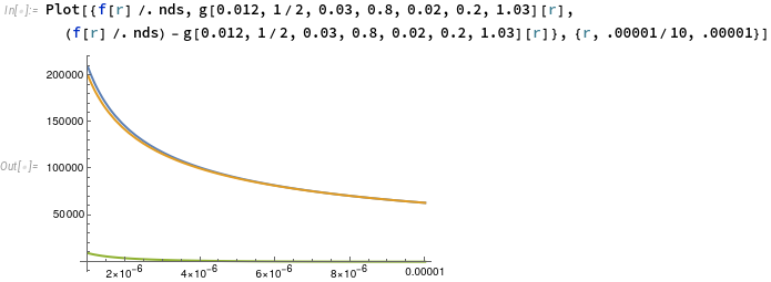
nds = Flatten@solver[.00001]

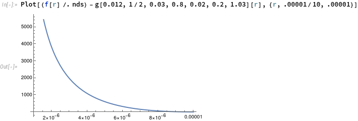
Here are f,g, and f-g:

Since the scales are quite different, here's f-g alone:

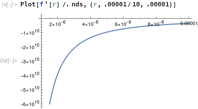
Here's f'[r]

[

And here are {{f[rSol],g[rSol]}{f'[rSol],g'[rSol]}}. f,g and f',g' are equal at rSol, as required.

{f[r] /. nds, 
   g[0.012, 1/2, 0.03, 0.8, 0.02, 0.2, 1.03][r]}, {f'[r] /. nds, 
   D[g[0.012, 1/2, 0.03, 0.8, 0.02, 0.2, 1.03][r], r]}} /. 
 r -> 9.999999999999999`*^-6

Out[53]= {{63245.6, 63245.6}, {-3.16228*10^9, -3.16228*10^9}}

Answer 3

We can map $(0, R)$ on $(0,1)$ using substitution $r\rightarrow R r$, and use ParametricNDSolveValue as follows

eq = 2 (\[Beta] f[r] + 
      r (-\[Mu] + \[Rho]) f'[
        r] + ((-1)^(\[Gamma]/(-1 + \[Gamma])) (R r)^((2 \[Gamma])/(-1 \
+ \[Gamma])) (-1 + \[Gamma]) \[Zeta]^(-(\[Gamma]/(-1 + \[Gamma]))) \
\[Rho]^(\[Gamma]/(-1 + \[Gamma])) (f'[r]/
            R)^(\[Gamma]/(-1 + \[Gamma])))/\[Gamma]) - 
   r^2 \[Sigma]^2 f''[r];


CONS = {\[Rho] -> 0.02, 
  J -> 5, \[Gamma] -> 0.5, \[Mu] -> 0.03, \[Sigma] -> 0.2, \[Zeta] -> 
   0.5, \[Beta] -> 0.012, k -> 10, \[Eta] -> 0.8, \[Lambda] -> 1.03}; 
g[r_] := (2^(1 - \[Gamma]) (1/R/
        r)^\[Gamma] \[Eta]^\[Gamma] \[Rho]^-\[Gamma] ((-2 \[Beta] + \
\[Gamma] (-2 \[Mu] + 
             2 \[Rho] + (1 + \[Gamma]) \[Sigma]^2))/(-1 + \
\[Gamma]))^(-1 + \[Gamma]))/\[Gamma] /. CONS;

sol = ParametricNDSolveValue[{eq == 0, f[1] == g[\[Lambda]], 
    f'[1] == \[Lambda] g'[\[Lambda]]} /. CONS, f, {r, 10^-3, 1}, {R}];

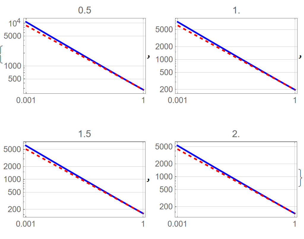
Visualization numerical solution (solid line) and function $g(\lambda r)$ (dashed red line) for R=0.5,1,1.5,2

Table[Show[
  LogLogPlot[sol[R][r], {r, 10^-3, 1}, PlotStyle -> Blue, 
   PlotLabel -> R, Frame -> True, GridLines -> Automatic, 
   FrameTicks -> {{Automatic, None}, {{0.001, 1}, Automatic}}], 
  LogLogPlot[g[\[Lambda] r] /. CONS, {r, 10^-3, 1}, 
   PlotStyle -> {Red, Dashed}]], {R, .5, 2, .5}]

Update 1. To satisfier condition at $r\rightarrow 0$ we suppose that $f(r)=a/r^{\gamma}$, and using eq we can define a as follows

rule = {f[r] -> a/r^\[Gamma] , f'[r] -> -\[Gamma]  a/r^(\[Gamma] + 1),
    f''[r] -> \[Gamma]  (\[Gamma] + 1) a/r^(\[Gamma] + 2)};

eq /. rule /. \[Gamma] -> 1/2 // FullSimplify; sl = Solve[% == 0, a];

Then we define function

f0 = a/r^\[Gamma] /. sl[[2]] /. CONS

Out[]= 158.114/(r^0.5 Sqrt[R])

Analyzing picture above we can suggest that function f0+b, where b is some constantan, should correlate with solution sol. To verifier this suggestion we use NMinimize as follows

eqn = (f0 + b - sol1[R][r]) /. r -> 10^-3;

 NMinimize[{eqn^2, {R > 0}}, {R, b}]

(*Out[]= {2.42103*10^-14, {R -> 138.914, b -> 215.84}}*)