1
$\begingroup$

I have a set of data points. The first coordinate is time and the second coordinate is energy. I am trying to figure out how the energy is decaying over time. Particularly, I have to find if it is decaying over time exponentially or as a power law. I used Mathematica FindFit to model my points as both an exponential decay and a power law decay. It turned out that the exponential decay describes my data points better. But I am not sure if I am doing the right thing. I also plotted my data points in a ListLogPlot and ListLogLogPlot. In both cases, I got a straight line. So, I am a little confused about the actual behavior of my data points. Could anyone help me with this issue? I am copying my data points here. Note that I am only interested in the late-time behavior of the function, not the entire time axis. Thank you!

Data1={{5,0.0210796},{7,0.0293022},{9,0.0302858},{11,0.0257149},{13,0.0182589},{15,0.0106745},{17,0.00473577},{19,0.00101295},{21,-0.000754187},{23,-0.00117344},{25,-0.000860244},{27,-0.000278088},{29,0.000293337},{31,0.00072545},{33,0.000988823},{35,0.00110603},{37,0.00111822},{39,0.00106582},{41,0.000980234},{43,0.000882181},{45,0.000783367},{47,0.000689278},{49,0.0006018},{51,0.000521108},{53,0.000446822},{55,0.000378596},{57,0.000316303}, {59, 0.000259989190761133}}

$\endgroup$
3
  • $\begingroup$ This doesn't seem like a Mathematica issue but rather a subject matter/statistics issue as you aren't having any issues with your Mathematica code. Maybe CrossValidated would be a better forum (stats.stackexchange.com). You should also mention exactly what you mean by "late-time behavior". $\endgroup$
    – JimB
    Commented Apr 11, 2023 at 23:38
  • $\begingroup$ @JimB What I mean by late-time behavior is that the time dependence of function at large times. For example after 30. $\endgroup$
    – HadamardN2
    Commented Apr 12, 2023 at 1:14
  • $\begingroup$ Thanks. Not everyone has the same idea about what constitutes "late-time behavior." Maybe I'm being too picky but I would expect you as knowledgeable about the subject matter to either have a particular and expected theoretical function and time threshold in mind. I don't see "For example after 30" sounding very definite. $\endgroup$
    – JimB
    Commented Apr 12, 2023 at 4:14

2 Answers 2

2
$\begingroup$

NonlinearModelFit (using exponential weights) gives an idea about longtimebehavior

Try

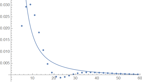
fit = NonlinearModelFit[data1, a + b/t ^c, {a, b, c}, t,Weights -> E^data1[[All, 1]]]  

enter image description here

Show[{ListPlot[data1], Plot[fit[t], {t, 0, 59}]}]

enter image description here

addendum

Thanks @MariuszIwaniuk

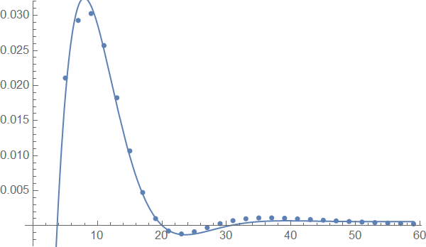
fitt = NonlinearModelFit[
  data1 , { a +   b Cos[c t + d] Exp[-e t]  , -Pi < d < Pi}, {   a,  
   b, c, d, e}, t, Weights ->  E^   Sqrt[data1 [[All, 1]]] , 
  Method -> "NMinimize"  ]

Show[{ListPlot[data1], Plot[fitt[t], {t, 0, 59}]}]

enter image description here

$\endgroup$
2
  • $\begingroup$ Maybe better is: NonlinearModelFit[data1, a + Exp[-b*t + c] Sin[d t + e], {{a, 5/1000}, b, c, {d, 1/7}, e}, t] ? $\endgroup$ Commented Aug 15 at 9:18
  • $\begingroup$ @MariusIwaniuk Keeping the weights-idea perhaps fit = NonlinearModelFit[ data1 , { a + b Cos[c t + d] Exp[-e t] , e > 0, -Pi < d < Pi}, { a, b, c, d, e}, t, Weights -> E^ Sqrt[data1 [[All, 1]] ], Method -> "NMinimize" ] $\endgroup$ Commented Aug 15 at 10:02
1
$\begingroup$

Not sure if this quite gives what you want, but by trial and error I can get a pretty good analytic approximation in terms of oscillating exponentials using Prony's method. There are a handful of posts here and on Wolfram Community where the code I'll show can be found, for example this MSE thread and this similar Community thread

The main caveat is that it is not obvious how many frequencies to retain; I use 5 because that seemed to give a very good fit. But quite possibly it is an overfit and would not be so close if more data points were available.

data1 = {{5, 0.0210796}, {7, 0.0293022}, {9, 0.0302858}, {11, 
    0.0257149}, {13, 0.0182589}, {15, 0.0106745}, {17, 
    0.00473577}, {19, 
    0.00101295}, {21, -0.000754187}, {23, -0.00117344}, {25, \
-0.000860244}, {27, -0.000278088}, {29, 0.000293337}, {31, 
    0.00072545}, {33, 0.000988823}, {35, 0.00110603}, {37, 
    0.00111822}, {39, 0.00106582}, {41, 0.000980234}, {43, 
    0.000882181}, {45, 0.000783367}, {47, 0.000689278}, {49, 
    0.0006018}, {51, 0.000521108}, {53, 0.000446822}, {55, 
    0.000378596}, {57, 0.000316303}, {59, 0.000259989190761133}};

timescale = 2;
start = data1[[1, 1]];
end = data1[[-1, 1]];
len = Length[data1];
vals = data1[[All, 2]];
mat = Most[Partition[vals, Floor[len/2], 1]];
keep = 5;
mat2 = Most[Partition[vals, keep, 1]];
rhs = Drop[vals, keep];
soln = PseudoInverse[mat2] . rhs;
roots = xx /. 
   NSolve[xx^keep - soln . xx^Range[0, keep - 1] == 0, xx];
freqs = Log[roots]

(* Out[678]= {-0.669853 - 0.858488 I, -0.669853 + 
  0.858488 I, -0.347502 - 0.431274 I, -0.347502 + 
  0.431274 I, -0.0686409} *)

newmat = Map[roots^# &, Range[start, end, timescale]/timescale];
coeffs = Chop[PseudoInverse[newmat] . vals, 10^(-5)];
newf0 = Chop[TrigExpand[ExpToTrig[coeffs . Exp[freqs*t/timescale]]]]

(* Out[681]= 
0.00310127 Cosh[0.0343205 t] - 
 0.125817 Cos[0.215637 t] Cosh[0.173751 t] + 
 0.0427935 Cos[0.429244 t] Cosh[0.334927 t] + 
 0.110279 Cosh[0.173751 t] Sin[0.215637 t] + 
 0.0447615 Cosh[0.334927 t] Sin[0.429244 t] - 
 0.00310127 Sinh[0.0343205 t] + 
 0.125817 Cos[0.215637 t] Sinh[0.173751 t] - 
 0.110279 Sin[0.215637 t] Sinh[0.173751 t] - 
 0.0427935 Cos[0.429244 t] Sinh[0.334927 t] - 
 0.0447615 Sin[0.429244 t] Sinh[0.334927 t] *)

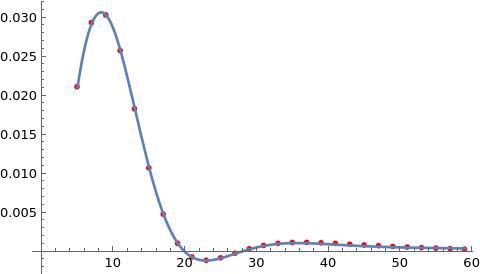
Here is a visual check.

pl = Plot[newf0, {t, start, end}];
lp = ListPlot[Style[data1, Red]];
Show[{lp, pl}]

enter image description here

$\endgroup$

Your Answer

By clicking “Post Your Answer”, you agree to our terms of service and acknowledge you have read our privacy policy.

Not the answer you're looking for? Browse other questions tagged or ask your own question.