8
$\begingroup$

Consider the following data:

TableDat = {{0.1, 0.1}, {0.2, 0.3}, {0.3, 0.55}, {0.5, 1}, {0.6, 
    1.17}, {0.8, 1.5}, {0.9, 1.6}, {1, 1.5}, {1.1, 1.3}, {1.25, 
    1.}, {1.35, 0.8}, {1.5, 0.5}};
ListPlot[TableDat]

I would like to fit it with a smooth function:

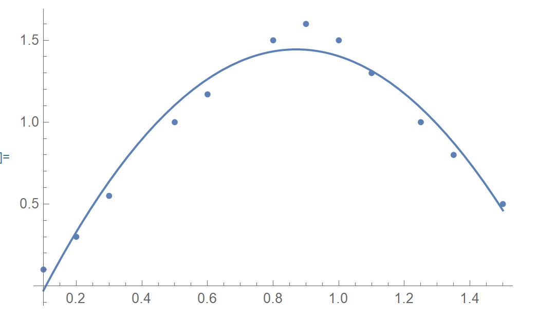
fit = NonlinearModelFit[TableDat, a*x + b*x^2 + c, {a, b, c}, x]
Show[Plot[fit[x], {x, 0.1, 1.5}], ListPlot[TableDat]]

enter image description here

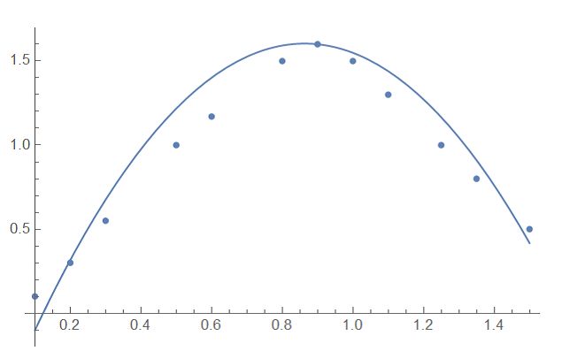
However, additionally, I want the value of the fitting function at x = 0.9 to match the data exactly. Is there a possibility to modify NonlinearModelFit to include this condition? A naive way would be to manually express c as a function of a,b from the condition a*x+b*x^2+c==1.6 at x = 0.9, but what about an automated way?

$\endgroup$

2 Answers 2

13
$\begingroup$

Just add a constraint

fit = NonlinearModelFit[TableDat, {a*x + b*x^2 + c, 
1.6 == (a*x + b*x^2 + c /. x -> 0.9)}, {a, b, c}, x]
Show[Plot[fit[x], {x, 0.1, 1.5}], ListPlot[TableDat]]

enter image description here

Hope it helps!

$\endgroup$
6
  • $\begingroup$ Just for reference: It is almost always a bad idea to save diagrams as JPG images, since the lossy JPG compression algorithm, which is designed for photographic images, causes rather visible and disturbing artefacts in non-photographic images. $\endgroup$ Commented Feb 9, 2023 at 14:01
  • $\begingroup$ @AndreasRejbrand Where did I save an image??? $\endgroup$ Commented Feb 9, 2023 at 15:19
  • $\begingroup$ Your third paragraph is a diagram saved as a JPG image! The artefacts are clearly visible around the axis labels, tick marks, and the curve, for instance. $\endgroup$ Commented Feb 9, 2023 at 17:57
  • $\begingroup$ @AndreasRejbrand I didn't understand your hint. Show gives a Graphics-object, Mathematica representation follows by ??Show[....], nothing saved as jpg $\endgroup$ Commented Feb 10, 2023 at 10:00
  • $\begingroup$ My apologies for being unclear. Your answer to this question contains four paragraphs: (1) "Just add a constraint", (2) a three-line code block in the Mathematica language, (3) an image of a scatter plot and an approximating curve, and (4) "Hope it helps!". When I first scrolled through this page, I stopped at the image mentioned above, because I am slightly autistic and therefore detect details very clearly, and this image has clear JPG artefacts, especially near the axis labels, tick marks, and the curve. $\endgroup$ Commented Feb 10, 2023 at 10:07
10
$\begingroup$

The right way

You say your model is

model = ( y == a*x + b*x^2 + c )

that is, three free parameters {a,b,c}.

But in reality, given the constraint { 0.9, 1.6 } your model has only two parameters {a,b}

model2 = FullSimplify[
    model/. First@Solve[ model /. { x -> 0.9, y -> 1.6 }, c ]
]

enter image description here

$PlotTheme = {"Scientific", "LargeLabels", "BoldScheme","DarkColor"};
fit = NonlinearModelFit[
    tableDat
    , Last@model2
    , {a, b}
    , x
    ];
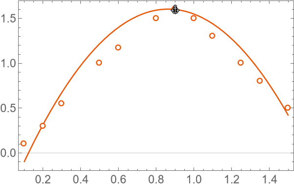
Show[
    Plot[
        fit[x]
        , {x, 0.1, 1.5}
    ]
    , ListPlot[tableDat]
    , Epilog -> Inset["⚓",{ 0.9, 1.6 }]
]

enter image description here

After @JimB's comment

Note that while the estimates for the slope and intercept don't change if one leaves in {0.9, 1.6}, the values for many of the summary statistics ("EstimatedVariance", "AIC", "AICc", "ParameterTable", etc,) differ depending on if one keeps or removes that one data point. I'd argue that if the choice the fixed point is selected from the observed points (as opposed to knowing that fixed point beforehand), I'd leave out that point to obtain more proper summary statistics.

therefore use

fit = NonlinearModelFit[
    DeleteCases[tableDat,  {0.9, 1.6}]
    , Last@model2
    , {a, b}
    , x
    ];

Your way

I would say that the previous solution is the correct way to do it, but given that you ask differently, refer to the answer by @UlrichNeumann (+1).

$\endgroup$
2
  • 2
    $\begingroup$ +1 for the anchor! (And I'd give another +1 for your "the right way" answer if that were possible.) Note that while the estimates for the slope and intercept don't change if one leaves in {0.9, 1.6}, the values for many of the summary statistics ("EstimatedVariance", "AIC", "AICc", "ParameterTable", etc,) differ depending on if one keeps or removes that one data point. I'd argue that if the choice the fixed point is selected from the observed points (as opposed to knowing that fixed point beforehand), I'd leave out that point to obtain more proper summary statistics. $\endgroup$
    – JimB
    Commented Feb 8, 2023 at 17:20
  • $\begingroup$ @JimB Thanks for the comment, I have edited my answer to quote your remark. $\endgroup$
    – rhermans
    Commented Feb 9, 2023 at 11:49

Your Answer

By clicking “Post Your Answer”, you agree to our terms of service and acknowledge you have read our privacy policy.

Not the answer you're looking for? Browse other questions tagged or ask your own question.