2
$\begingroup$

I have already asked a similar question regarding approximating Taylor series of the function from noisy data. This is another example I am having trouble with. Consider the integral $$I(x)=\int_0^1\frac{(1-y)^{5/6}y^{3/4}}{x+1-y^{15/4}}dy$$ for small $x>0$. I put specific exponents $15/4$ and $3/4$ but they are not important. What is important is the fractional exponent $5/6$, then the series expansion of $I(x)$ has the form $$ I(x) =x^{5/6}(a_0+a_1 x+a_2 x^2+\ldots) + b_0+b_1 x+b_2 x^2+\ldots. $$ This behaviour follows from simple arguments. First, near $y=0$ the integral is well behaved and regular in $x$ for small $x$. Near $y=1$ we make a change of variables $y=1-t$ and can approximate a contribution from $y\approx 1$ as $$\int_0^1 \frac{t^{5/6+k}}{t+x}dt,\quad k=0,1,\ldots$$ This integral can be evaluated in Mathematica in terms of $\phantom{l}_2F_1$. The expansion of $\phantom{l}_2F_1$ produces the above series.

Obviously, we can numerically calculate $I(x)$ for small $x>0$ with any precision.

${\bf Question}$: How to find accurate values for coefficients $a_i$, $b_i$, say for $i=1,\ldots,10$ ?

An ``obvious'' way is to make a change of variable $x=z^6$. Then $I(z^6)$ becomes a polynomial in $z$ and we could use the Cauchy formula to evaluate coefficients of $I(z^6)$ as contour integrals about $z=0$ $$\frac{1}{2\pi i}\oint_{C_0} \frac{dz}{z^{k+1}}I(z^6)$$

Unfortunately, this fails because the integral $I(x)$ converges only for $x>0$ and the Cauchy integral requires all complex values of $x$ near $0$ including $x<0$.

I can't think of any other analytic method. Surely, it can be done by fitting $I(x)$ for sufficiently many points $x_i$. However, I again meet the problem of growing high coefficients in the series expansion coming from truncation. I am not an expert in numerical analysis. Can anyone help with this specific example?

Code example :

F[x_] := NIntegrate[(1 - y)^(5/6)*y^(3/4)/(x + 1 - y^(15/4)), {y, 0, 1}, 
WorkingPrecision -> 20];

 data = Array[{#/500, F[#/500]} &, 50];
 
fun0=Array[x^(# - 1) &, 10]; funs = Union[x^(5/6)*fun0, fun0]; 

result=Fit[data, funs, x]


N[result]=0.327029 - 0.556915 x^(5/6) + 0.233352 x + 0.467191 
x^(11/6) - 0.242948 x^2 - 0.411222 x^(17/6) + 0.23187 x^3 + 0.430319 
x^(23/6) - 0.341292 x^4 + 3.08767 x^(29/6) - 6.02764 x^5 + 86.0805 
x^(35/6) - 134.697 x^6 + 865.519 x^(41/6) - 1158.21 x^7 + 3151.6 
x^(47/6) - 3480.96 x^8 + 3016.48 x^(53/6) - 2494.16 x^9 + 156.266 
x^(59/6) 

One can add more points to the data set but higher coefficients are not stable.

Update: I realised that the problem is reduced to fitting a normal Taylor series. It is possible to isolate explicitly a fractional power $x^{5/6}$ in this integral by a slight change of variable $x\to (1+x)^{15/4}-1\approx \frac{15}{4}x+\ldots$. Introduce $$ J(x)=I((1+x)^{15/4}-1)=\int_0^1\frac{(1-y)^{5/6}y^{3/4}}{(x+1)^{15/4}-y^{15/4}}dy=\frac{8\pi}{15}\frac{x^{5/6}}{(1+x)^2}+b(x) $$

$$b(x)=b_0+b_1 x+b_2 x^2+\ldots.$$

The proof of such expansion is done using dispersion relations. The problem of growing coefficients in the series remains.

$\endgroup$
5
  • $\begingroup$ Are you sure you posted this on the appropriate StackExchange site? It looks like you are trying to find an analytic method, therefore this is more appropriate for the Mathematics StackExchange. This site is dedicated only to the software Wolfram Mathematica. $\endgroup$
    – Domen
    Commented Sep 13, 2022 at 13:24
  • $\begingroup$ I am not trying to find another analytic method, I doubt that it exists. It is a numerical question, I only need numerical values of coefficients in the series. And I do all fitting in Mathematica, so is my question here. $\endgroup$
    – VladM
    Commented Sep 13, 2022 at 13:33
  • $\begingroup$ In that case, please provide some Mathematica code for the presented integrals. Otherwise, my naive approach would be to generate a table of values for $I(x)$, and then fit your polynomial ansatz by (Non)linearModelFit to those points ... I guess that with sufficiently enough points, this should converge to true coefficients ... $\endgroup$
    – Domen
    Commented Sep 13, 2022 at 13:47
  • $\begingroup$ The integral contains (1-y)^(5/6) and you wrote (1-y^(5/6)). Yours is a much simpler integral. $\endgroup$
    – VladM
    Commented Sep 15, 2022 at 14:17
  • $\begingroup$ Since you found a way to substract the non analytical part, why not use Needs["NumericalCalculus`"]; ND[analytical part,{x, n},0,Method->NIntegrate] (and maybe adjust the radius of the circle on which the Cauchy integral is done) ? $\endgroup$ Commented Sep 15, 2022 at 17:05

4 Answers 4

1
$\begingroup$

Interestingly, Taylor originally developed what we now call the Taylor series by taking the limit of an interpolation of the function as the interpolation nodes approached the center of the power series. We can do the same thing on F[u^6]. Using a regular partition seems to run into the Runge phenomenon, if I try to get a series higher than around degree $x^4$. Ultimately, I had to bump the working precision quite high and use a Chebyshev interpolation. Even with that, converting to a power basis to get the Taylor coefficients lost most of the advantage over a regularly spaced nodes.

It takes a fairly long time (470 sec., almost 8 min.) -- I forgot to time it.

F // ClearAll;
F[x_] := F[x] =
   NIntegrate[(1 - y)^(5/6)*y^(3/4)/(x + 1 - y^(15/4)),
    {y, 0, 1},
    WorkingPrecision -> 200, (* reduce for faster & less accurate *)
    Method -> {"GaussKronrodRule", "Points" -> 41}, 
    MaxRecursion -> 30];

deg = 128;
chebnodes = Rescale[Sin[Pi/2 Range[-deg, deg, 2]/deg]]/4;
yvals = F[#^6] & /@ chebnodes;

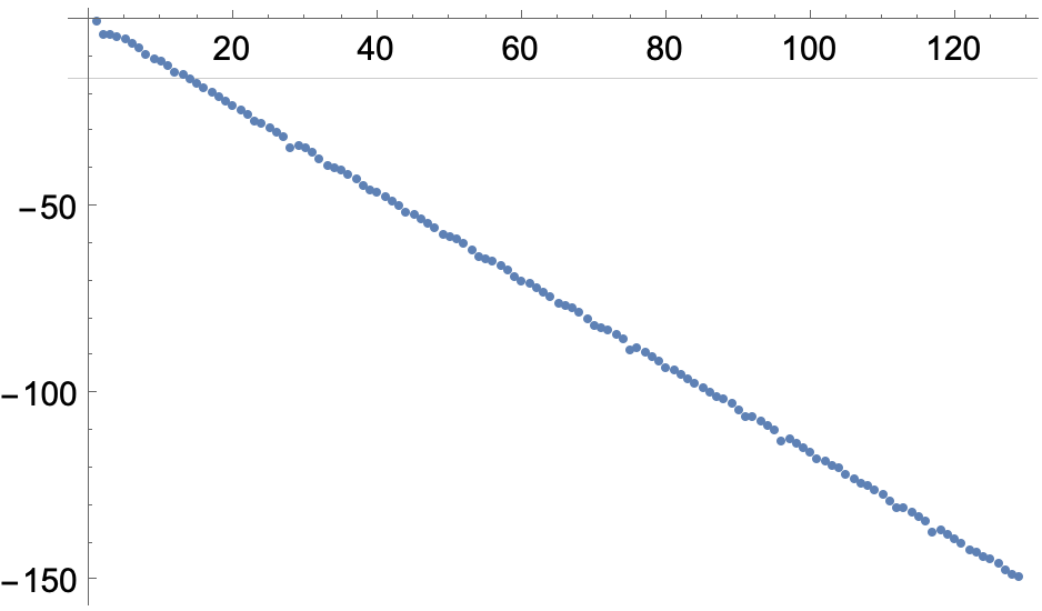
(* optional: check quality of approx.: *)
chebcoeffs = Sqrt[2/deg] FourierDCT[yvals, 1];
chebcoeffs[[{1, -1}]] /= 2;
ListPlot[RealExponent[chebcoeffs]]

About 150 digits of accuracy if evaluated carefully. Of course, we're expanding in power-series form, which numerically is not being careful at all. In the expansion of the interpolating polynomial, precision is lost as the degree goes up.

Statistics`Library`BarycentricInterpolation[
 N[chebnodes, 1000],  yvals][x^(1/6)] //
  Together // Expand // N[#, 20] &
(*
 0.32702920805305913492     - 0.55691537891020777360 x^(5/6) + 
 0.23335188357873085006 x   + 0.46719012341911874341 x^(11/6) - 
 0.24294583606336861750 x^2 - 0.41159312363254260008 x^(17/6) + 
 0.23279014838185126923 x^3 + 0.37345608624294385863 x^(23/6) - 
 0.22141853884387890746 x^4 - 0.34517607282363951340 x^(29/6) + 
 0.21110850199135615504 x^5 + 0.32307531917592692889 x^(35/6) - 
 0.20206988221563788298 x^6 - 0.30515142767493422917 x^(41/6) + 
 0.19415974155731052088 x^7 + 0.29021067477272687801 x^(47/6) - 
 0.18719408481478643888 x^8 - 0.27749113076195189203 x^(53/6) + 
 0.18101051230728878713 x^9 + 0.26648016601623575 x^(59/6) - 
 0.1754767983601454 x^10    - 0.25681819010 x^(65/6) + 
 0.1704874308 x^11          + 0.24824 x^(71/6) -
 0.1660 x^12
*)
$\endgroup$
0
$\begingroup$

I have no idea whether this approach is mathematically valid, but I'll post it anyway. As suggested in the comments, tabulate your integral and use NonlinearModelFit.

f[x_] := NIntegrate[(1 - y)^(5/6)*y^(3/4)/(x + 1 - y^(15/4)), {y, 0, 
    1}];
data = Table[{x, i[x]}, {x, 0, 10, 0.0001}];

fit[aN_, bN_] := Module[{as, bs},
  as = a /@ Range[0, aN];
  bs = b /@ Range[0, bN];
  NonlinearModelFit[data, 
   x^(5/6) (as . x^Range[0, aN]) + (bs . x^Range[0, bN]), as~Join~bs, 
   x]
  ]

(* Expansion up to 6th term in both a and b *)
fit[5, 5][x]

(* 0.326974 + 0.183902 x - 0.720627 x^2 + 0.51628 x^3 + 0.184807 x^4 + 
 0.00682896 x^5 + 
 x^(5/6) (-0.532243 + 0.87208 x - 0.434412 x^2 - 0.259422 x^3 - 
    0.0139618 x^4 - 0.0000271934 x^5) *)


Show[ListPlot[data, PlotRange -> All], 
 Plot[Evaluate[fit[10, 10][x]], {x, 0, 10}, PlotStyle -> Red, 
  PlotRange -> All]]

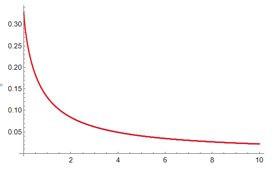
enter image description here

Do coefficients converge?

Row[Table[
  ListPlot[Table[Coefficient[fit[n, n][x], x, k], {n, 1, 30}], 
   PlotLabel -> b[k], ImageSize -> 300, Frame -> True], {k, 0, 3}]]

enter image description here

$\endgroup$
1
  • $\begingroup$ You can not use large x for your fit and truncate at low powers. If you truncate at x^n, you expect that b_{n+1}*x^{n+1} should be roughly your error for all points in the data set. In your case n=5 and for x=10 0.00682896 x^5 = 70. It means that x^6 will make a large contribution and your coefficients are far from true values. In addition, coefficients should be stable for different data sets. $\endgroup$
    – VladM
    Commented Sep 13, 2022 at 14:31
0
$\begingroup$

As the exponents of y are not important, we can as well set them to "1" to make things simpler. Then:

f[x_] := Integrate[(1 - y)^(5/6)*y/(x + 1 - y), {y, 0, 1}];

And the series will be:

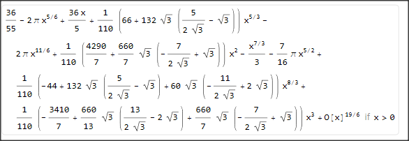
Series[f[x], {x, 0, 3}]

enter image description here

$\endgroup$
1
  • $\begingroup$ When I said "not important", I meant that they do not change the form of asymptotics, only the coefficients of the expansion. Of course, if you set them to zero, the integral becomes trivial and can be calculated in a closed form. In my real problem, they are 15/4 and 3/4, but they should not matter for for a numerical method. $\endgroup$
    – VladM
    Commented Sep 13, 2022 at 22:59
0
$\begingroup$

Since the problem reduced to finding accurate coefficients in Taylor series, I think the best method is to use difference derivatives. It worked well in my case and the ND function produced some nonsense.

I give the general formula here which I found in B. Fornberg, SIAM Review 40, 685-691. The $n$-th derivative of the function $f(x)$ at $x=x_0$ can be calculated from

$$D_n[f(x_0)]=\frac{d^n}{dx^n}f(x)|_{x=x_0}=\frac{1}{h^n}\sum_{k=-s}^{m-s} a_kf(x_0+kh)$$

where the coefficients $a_k$ are defined from series $$ \sum_{k=-s}^{m-s}a_k x^{k+s}=\sum_{j=0}^m\frac{(x-1)^j}{j!}\frac{d^j}{dy^j}(y^s(\log y)^n)|_{y=1}$$

Here $h$ is a step, $m$, $s$ are integer parameters. For left derivatives you take $m=s$, for right derivatives you take $s=0$, for central derivatives you take $m=2s$. Choosing sufficiently large values $m$, $s$ and small steps, you can evaluate derivatives with arbitrary accuracy. Of course, you need to know the function with the same accuracy.

Example: $n=2$, $x_0=0$, $s=0$, $m=5$. The above formula produces

$$D_2[f(0)]=\frac{1}{h^2}\left(\frac{15}{4}f(0)-\frac{77}{6}f(h)+\frac{107}{6}f(2h)-13f(3h)+\frac{61}{12}f(4h)-\frac{5}{6}f(5h)\right)$$

Expanding the above expression in series produces $$D_2[f(0)]=f''(0)-\frac{137}{180}f^{(6)}(0)h^4+\ldots$$, i.e. the error is of the order $h^4$.

Code:

acoffs[n_, m_] := Module[{mu}, 
mu = Expand[Sum[((x - 1)^j*(Together[D[Log[y]^n, {y, j}]] /. y -> 1))/j!, 
         {j, 0, m}]]; Array[a[#1 - 1] -> Coefficient[mu, x, #1 - 1] & , m + 1]]

Taylor[f_, n_, m_, h_] := (1/(h^n*n!))*Sum[f[k*h]*a[k], {k, 0, m}] /. 
     acoffs[n, m]

JJ[x_] := NIntegrate[((1 - t)^(5/6)*t^(3/4))/(t^(15/4) - (1 + x)^(15/4)), 
      {t, 0, 1}, WorkingPrecision -> 100, MaxRecursion -> 50] - 
     8*(Pi/15)*(x^(5/6)/(1 + x)^2)

N[Sum[Taylor[JJ, i, 20, 1/100000]*x^i, {i, 0, 10}], 20]

-0.32702920805305913492 - 0.87506956342024068774 x + 
 2.2132051699382902379 x^2 - 3.5827506893877561559 x^3 + 
 4.9557979013187667467 x^4 - 6.3256682575303549939 x^5 + 
 7.6922703284511412126 x^6 - 9.0569502237776198146 x^7 + 
 10.420821546401807087 x^8 - 11.784465228324432941 x^9 + 
 13.148076408492987362 x^10
```
$\endgroup$
7
  • $\begingroup$ Please add the actual Mathematica code that answers the question. $\endgroup$
    – bbgodfrey
    Commented Sep 16, 2022 at 5:59
  • $\begingroup$ @VladM: Could you please post your series expansion of $I(x)$ say to 10 terms? I'm looking at another approach. $\endgroup$
    – josh
    Commented Sep 16, 2022 at 13:38
  • $\begingroup$ For the finite differences you can use DifferenceQuotient $\endgroup$ Commented Sep 17, 2022 at 19:20
  • $\begingroup$ I think the reason why ND with the option NIntegrate did not work is that the plot of the function JJ for x between -1 and 1 seems to be chaotic for negative x and so it does not look analytic around 0. Is there a reason why your forward finite differences only consider points for x>0 ? $\endgroup$ Commented Sep 17, 2022 at 20:01
  • $\begingroup$ I forgot to define functions to[..] and co[...] which are simply Together and Coefficient. I always define them to save time on typing. Now it should work. The integral for JJ(x) does not converge for x<0 because it has a logarithmic singularity at t=1+x, x<0. The analytic continuation of the integral has a branch cut (-infinity,0) coming from x^(5/6). This is the reason why I used only forward derivatives for x>0. Once you subtract the singularity x^(5/6) as it is done in JJ(x), the remaining part is regular at x=0. $\endgroup$
    – VladM
    Commented Sep 18, 2022 at 3:02

Your Answer

By clicking “Post Your Answer”, you agree to our terms of service and acknowledge you have read our privacy policy.

Not the answer you're looking for? Browse other questions tagged or ask your own question.