2
$\begingroup$

This is an immediate follow-up to DoAny--which I did consider editing, clarifying and correcting in some respects.

But perhaps here I can put the immediate question at hand more directly (the emphasis here is on "can fit", rather than "do fit"). Previously, I attempted to fit the CopulaDistributions by using the mathematical copula formulas in WikiCopulaArticle (rather than, more correctly, the probability distribution functions (PDF's)) of the CopulaDistribution commands themselves. So, I did not directly address the title question here before.

As before, I have two $50 \times 50$ matrices of counts (q1 and Q1 BivariateCopulaRepulsive), where the (i,j)-cell of each is parameterized by coordinates $x=\frac{2 i-1}{100}$ and $y=\frac{2 j-1}{100}$, $i,j = 1,\cdots,50$. The (i,j}-cell of q1 records the total number of counts for that cell, and Q1 only those counts that pass an additional "separability" (non-entanglement) test. Both $x$ and $y$ ("Bloch radii" in quantum/qubit parlance) lie in [0,1]. Due to complicated (random-matrix-based RandomMatrixProcedure) sampling procedures, it is not possible to (ideally) generate the same number of counts for each cell of q1, and we are, unfortunately, at least at this stage of sampling, left with numerous indeterminate cells.

Now, and this was not well clarified in the previous question and perhaps incorrectly put, I have strong (quantum-information-theoretic MarginalProbabilityInvariance InvarianceOfSeparabilityProbability) reasons for believing that the $50 \times 50$ scaled ratio-matrix $R= \frac{33 Q1}{4 q1}$ 50by50ScaledRatioMatrix

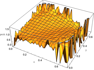
ScaledRatioMatrixPlot

should be well-fitted by a (symmetric around $x=y$) bivariate function $f(x,y) \in [0,1] \times [0,1]$, the univariate marginal distributions of which are uniform. In other words, the PDF of a "copula"--"a multivariate (bivariate, here) cumulative distribution function [CDF] for which the marginal probability distribution of each variable is uniform on the interval [0, 1]" WikiCopulaArticle.

To support the assertion of marginal uniformity, I indicate that the row/column sums of Q1 divided by the row/column sums of q1 are, respectively,

{0.122152,0.123213,0.124391,0.12561,0.124958,0.124737,0.124693,0.125091,0.124743,0.125195,0.124543,0.124235,0.123994,0.124222,0.123835,0.123876,0.123843,0.123646,0.123359,0.123083,0.122888,0.122807,0.122958,0.122107,0.122693,0.122233,0.121039,0.120738,0.121431,0.124553,0.126923,0.114433,0.117077,0.119403,0.0769231,Indeterminate,Indeterminate,Indeterminate,Indeterminate,Indeterminate,Indeterminate,Indeterminate,Indeterminate,Indeterminate,Indeterminate,Indeterminate,Indeterminate,Indeterminate,Indeterminate,Indeterminate}

and

{0.12248,0.125549,0.123342,0.124682,0.125103,0.124306,0.125221,0.124839,0.125349,0.124404,0.124586,0.124481,0.124217,0.124276,0.124066,0.123791,0.123513,0.123781,0.123269,0.123403,0.122808,0.123257,0.122091,0.122277,0.122445,0.121522,0.121564,0.120654,0.122414,0.122399,0.124401,0.119962,0.112939,0.137072,0.0555556,Indeterminate,Indeterminate,Indeterminate,Indeterminate,Indeterminate,Indeterminate,Indeterminate,Indeterminate,Indeterminate,Indeterminate,Indeterminate,Indeterminate,Indeterminate,Indeterminate,Indeterminate}.

Note that our theoretically-anticpated value of $\frac{4}{33}$ is $\approx 0.121212$.

It further appears that $x$ and $y$ are "repulsive", that is the probabilities for the line $x=y$ are relatively low BlochRadiiRepulsion.

Now, the question I would like to put is whether or not it is possible to fit the PDF's of the built-in Mathematica CopulaDistributions (or possibly not listed superior ones) to the indicated scaled ratio matrix R, providing estimates of the parameters of those distributions and measures of fit?

Ideally, the desired PDF's and CDF's could be obtained through direct integration--without the use of sampling and need for this question. However, the immediate problem under consideration is 14-dimensional in nature (being the rank-3 counterpart 14-dimensionalBoundaryTwo-Qubit to a full [15-dimensional] rank-4 problem 15-dimensional/Two-Qubit--also MarginalProbabilityInvariance InvarianceOfSeparabilityProbability)--so well beyond standard integration procedures.

$\endgroup$
0

2 Answers 2

3
$\begingroup$

The answer to “Can a copula distribution be used to describe the matrix of ratios $33 Q1/(4 q1)$? is technically “No.” Here is why I say that.

The matrix of ratios $Q1/q1$ are simply the estimates of the conditional probability of a single $q1(x,y)$ sample passing the separability test. The collection of the underlying true conditional probabilities is likely described by some continuous bivariate function but that bivariate function cannot be a bivariate probability distribution let alone a copula. (And multiplying that ratio by 33/4 does nothing to allow one to call that resulting bivariate function a probability density function.)

Now some functional form of a copula pdf (probability density function) might provide a reasonable description of the underlying bivariate function. If that pdf is given by $f(x,y)$, then maybe $a_0 + a_1 f(x,y)$ might work but none of the statistical properties of a bivariate pdf apply.

“To support the assertion of marginal uniformity, I indicate that the row/column sums of Q1 divided by the row/column sums of q1 are, respectively…” What you are doing is simply taking means across rows and columns and seeing that the resulting ratios (i.e., conditional probabilities of passing the separability test) are relatively constant and near your proposed theoretical value. There is nothing in that procedure that warrants stating that Uniform(0,1) probability distributions are involved.

$\endgroup$
1
$\begingroup$

Let us begin by trying to fit the Ali-Mikhail-Haque copula

d = CopulaDistribution[{"AMH", g}, {UniformDistribution[],UniformDistribution[]}]

where g is the unknown parameter. Further, we employ the function

c[g_,x_,y_] := Evaluate[PDF[d, {x, y}]]

Seeking a least-squares fit to the entries of R greater than 0, we employ

u = (2 i - 1)/100; v = (2 j - 1)/100; s = 0; Do[If[R[[i, j]] > 0, s = s + (c[g, u, v] - R[[i,j]])^2], {i, 1, 50}, {j, 1, 50}]; NMinimize[s, g]

yielding

{226.934, {g -> -0.180312}}.

Alternatively, weighting the (i,j) contribution to the sum by the original total counts for that cell--that is the (i,j) entry of the total count matrix q1--

u = (2 i - 1)/100; v = (2 j - 1)/100; s= 0; Do[If[R[[i, j]] > 0, s = s + q1[[i, j]] (c[g, u, v] - R[[i, j]])^2], {i,1, 50}, {j, 1, 50}]; NMinimize[s, g]

we obtain a contrastingly positive estimate of g,

{204800., {g -> 0.0192858}}.

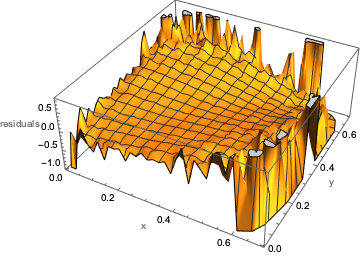
Here is a plot of the residuals of R from this fit

enter image description here

Further still, repeating the prior calculation, but replacing the square by the more robust absolute value function,

u = (2 i - 1)/100; v = (2 j - 1)/100; s = 0; Do[

If[R[[i, j]] > 0, s = s + q1[[i, j]] Abs[c[g, u, v] - R[[i, j]]]], {i, 1, 50}, {j, 1, 50}]; NMinimize[s, g]

we obtain a near-to-zero estimate of g,

{1.63462*10^6, {g -> 0.0125446}}.

Some ListPlot3D's of these various fits might now be in order.

We now anticipate similarly studying the other built-in CopulaDistributions, and seeking the best fits among them.

In fact, let us similarly examine a two-parameter Multinormal model. Then,

d = CopulaDistribution[{"Multinormal", {{g1, g2}, {g2, g1}}}, {UniformDistribution[], UniformDistribution[]}]; c4[g1_, g2_, x_,y_] := Evaluate[PDF[d, {x, y}]] u = (2 i - 1)/100; v = (2 j - 1)/100; s = 0; Do[If[R[[i, j]] > 0, s = s + q1[[i, j]] Abs[c4[g1, g2, u, v] - R[[i, j]]]], {i, 1,50}, {j, 1, 50}]; NMinimize[s, {g1, g2}]

yields

{1.6365*10^6, {g1 -> 0.396414, g2 -> 0.000843069}}

with the covariance parameter near to zero.

If we expand this two-parameter multinormal model to a three-parameter one

d = CopulaDistribution[{"Multinormal{{g1, g2}, {g2, g3}}}, {UniformDistribution[], UniformDistribution[]}]; c4[g1_, g2_, g3_, x_, y_] :=Evaluate[PDF[d, {x, y}]]; u = (2 i - 1)/100; v = (2 j - 1)/100; s = 0;Do[If[R[[i, j]] > 0, s = s + q1[[i, j]] Abs[c4[g1, g2, g3, u, v] - R[[i, j]]]], {i, 1, 50}, {j, 1, 50}]; NMinimize[s, {g1, g2, g3}]

we get the same goodness-of-fit result, but now

{1.6365*10^6, {g1 -> 2.5036, g2 -> 0.00281383, g3 -> 0.6992}}

I'm a little puzzled as to how to jointly interpret these last two outcomes--in light of the presumed symmetry between x and y.


In any case, the answer to the title question certainly seems to be

Yes.

$\endgroup$

Your Answer

By clicking “Post Your Answer”, you agree to our terms of service and acknowledge you have read our privacy policy.

Not the answer you're looking for? Browse other questions tagged or ask your own question.