The basic problem appears to be a convective-diffusive heat transfer problem of X-directed fluid flow across a heated spherical cap tip. To study this type of problem, it probably is easier to construct a virtual cuboid wind tunnel. When simulating virtual wind tunnels, the upstream section is typically much shorter than the downstream week region, so there really is not any spherical symmetry.
The following workflow will show how to construct a virtual wind tunnel and add refinement zones so that gradients may be captured near the object of interest without blowing up the total model size.
Virtual wind tunnel construction with refinement zones.
As discussed here, a MeshRefinementFunction will not necessarily refine the surface mesh in 3D. The suggested workaround was to use BoundaryDiscretizeRegion to obtain a finely discretized surface mesh on the input geometry before applying the MeshRefinementFunction.
The following workflow creates a refined region with a finely discretized tip and a wind tunnel domain less refined region:
<< NDSolve`FEM`
Pe = 15;
tip = BoundaryDiscretizeRegion[Ball[], MaxCellMeasure -> .00125,
Axes -> True, AxesLabel -> {"X", "Y", "Z"}];
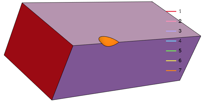
refCuboid =
BoundaryDiscretizeRegion[Cuboid[{-1.5, 0, -1.5}, {3.5, 1.5, -0.8}],
MaxCellMeasure -> .01, Axes -> True, AxesLabel -> {"X", "Y", "Z"}];
reftip = RegionDifference[refCuboid, tip, Axes -> True,
AxesLabel -> {"X", "Y", "Z"}]
domCuboid =
BoundaryDiscretizeRegion[Cuboid[{-2.5, 0, -3.8}, {7.5, 4, -0.8}],
Axes -> True, AxesLabel -> {"X", "Y", "Z"}];
domref = RegionDifference[domCuboid, refCuboid, Axes -> True,
AxesLabel -> {"X", "Y", "Z"}]
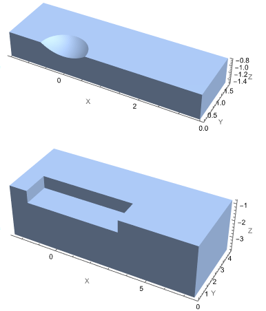
Create volume mesh with refinement zones
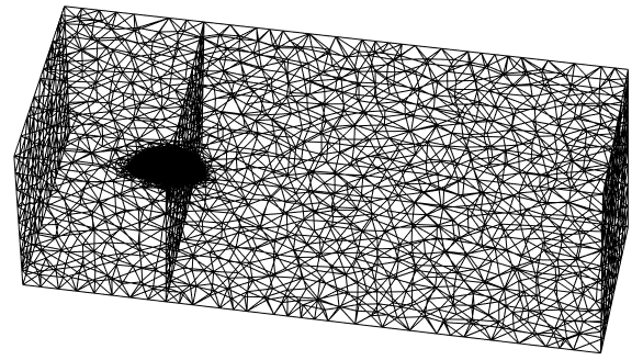
The following workflow creates a refinement zone with a high level of surface discretization at the tip. The total number of elements is about 134,000, which does not take too long to solve.
(* Create Mesh Refinement Function *)
mrf = With[{rmf = RegionMember[reftip]},
Function[{vertices, volume},
Block[{x, y, z}, {x, y, z} = Mean[vertices];
If[rmf[{x, y, z}], volume > (0.07/1.5)^3, volume > (0.3)^3]]]];
(* Create and Display Volumetric Mesh *)
mesh = ToElementMesh[RegionUnion[domref, reftip],
MeshQualityGoal -> "Maximal", "MeshElementConstraint" -> 40,
"MaxBoundaryCellMeasure" -> {"Length" -> .1},
MeshRefinementFunction -> mrf]
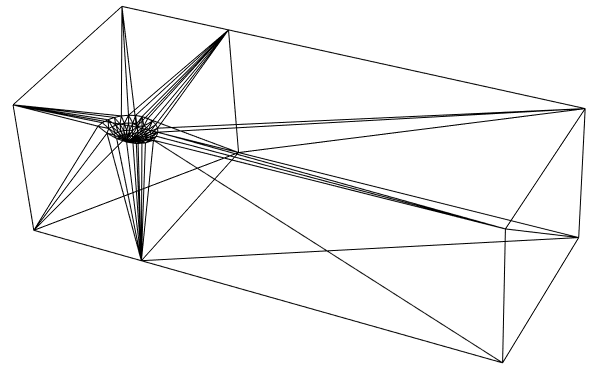
mesh["Wireframe"[
"MeshElement" -> "MeshElements",
"ElementMeshDirective" -> Directive[EdgeForm[Black]],
PlotRange -> {{-2.5`, 7.5`}, {0.2,
4.`}, {-3.8`, -0.7999999999999998`}}]]
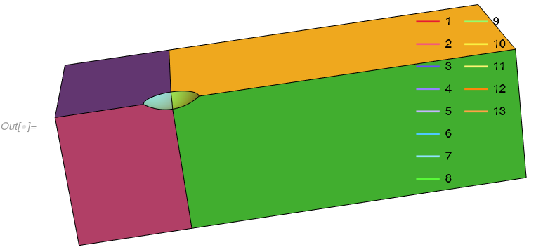
groups = mesh["BoundaryElementMarkerUnion"];
temp = Most[Range[0, 1, 1/(Length[groups])]];
colors = ColorData["BrightBands"][#] & /@ temp
mesh["Wireframe"["MeshElementStyle" -> FaceForm /@ colors]]
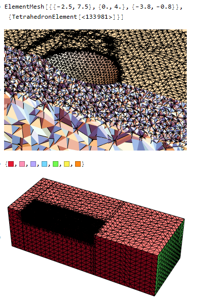
Solution
We and solve and now compare our solution on the refined mesh versus the OP mesh.
sol = NDSolveValue[{D[T[x, y, z], x] ==
1/Pe Laplacian[T[x, y, z], {x, y, z}], {DirichletCondition[
T[x, y, z] == 1., ElementMarker == 3],
DirichletCondition[T[x, y, z] == 0., ElementMarker == 4]}},
T, {x, y, z} ∈ mesh];
z1 = -0.8;
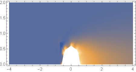
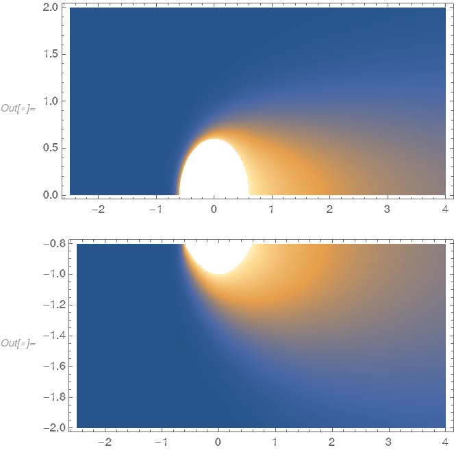
DensityPlot[sol[x, y, z1], {x, -4, 4}, {y, 0, 2}, PlotRange -> All,
 PlotPoints -> 100, AspectRatio -> 1/2]
DensityPlot[sol[x, 0, z], {x, -4, 4}, {z, -0.8, -2}, PlotRange -> All,
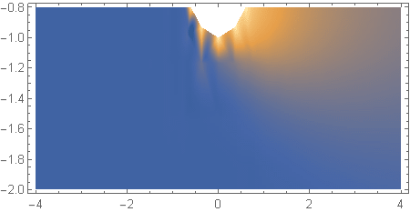
  PlotPoints -> 100, AspectRatio -> 1/2]
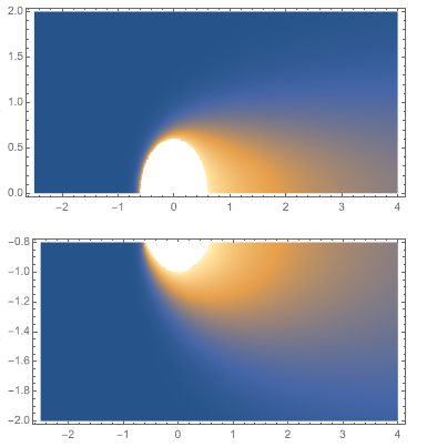
Visually, the solution appears to be much smoother than the images shown in the OP.
Other plots
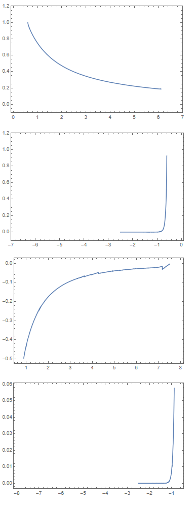
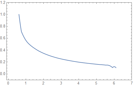
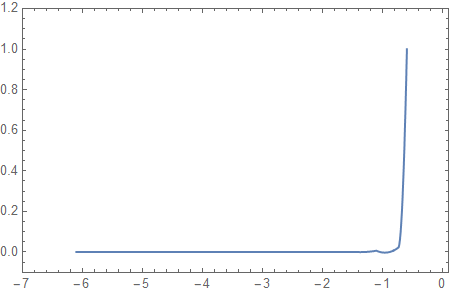
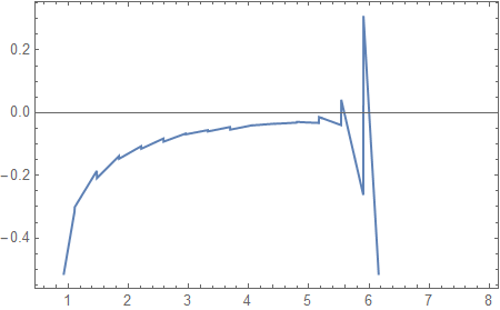
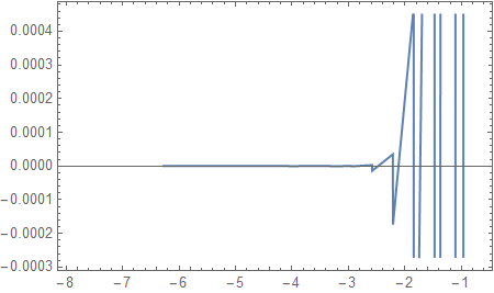
The other plots appear much smoother with the refined mesh.
Plot[sol[x, 0, -0.8], {x, 0.6, 6.1}, Frame -> True,
 PlotRange -> {{-0.1, 7}, {-0.1, 1.2}}]
Plot[sol[x, 0, -0.8], {x, -6.1, -0.6}, Frame -> True,
 PlotRange -> {{-7, 0.1}, {-0.1, 1.2}}]
Dr[x_, y_, z_] = D[sol[x, y, z], x];
Plot[Dr[x, 0, -0.8], {x, 0.6, 8}, Frame -> True]
Plot[Dr[x, 0, -0.8], {x, -8, -0.6}, Frame -> True]
Integration of total flux
The integration strategy given in the OP does solve albeit quite slowly due to slow convergence issues. When I evaluate the OP code, I obtained:
NIntegrate[#, {x, y, z} ∈ SC1] & /@ (Grad[
    sol[x, y, z], {x, y, z}] . {x, y, z})
NIntegrate[#, {x, y, z} ∈ SC2] & /@ (Grad[
    sol[x, y, z], {x, y, z}] . {x, y, z})
(* -0.95414 *)
(* -2.96035 *)
Summing up the discretized data
Using a variety of Mathematica functions, we can extract the normals, areas, and thermal gradients of each triangle on the mesh corresponding to the spherical cap. This should be enough information to estimate an integrated flux.
The following workflow shows how to extract the necessary information for the left and right-hand sides of the spherical cap.
(*Element info shortcuts*)
ebi = ElementIncidents[#["BoundaryElements"]][[1]] &;
ebm = ElementMarkers[#["BoundaryElements"]][[1]] &;
ebn = #["BoundaryNormals"][[1]] &;
ei = ElementIncidents[#["MeshElements"]][[1]] &;
em = ElementMarkers[#["MeshElements"]][[1]] &;
epi = ElementIncidents[#["PointElements"]][[1]] &;
epm = Flatten@ElementMarkers[#["PointElements"]] &;
(*extract boundary mesh from element mesh*)
bmesh = ToBoundaryMesh[mesh];
bcrd = bmesh["Coordinates"];
bi = ebi[bmesh];(*boundary element incidents*)
bm = ebm[bmesh];(*boundary element markers*)
bn = ebn[bmesh];(*boundary normals*)
(*find markers corresponding to the spherical cap*)
mrk3pos = Flatten@Position[bm, 3, 1];
(*generate necessary info to estimate surface integral*)
bn3 = bn[[mrk3pos]];
polys = Map[Polygon,
   GetElementCoordinates[bcrd, #] & /@ bi[[mrk3pos]]];
area3 = Area /@ polys;
center3 = Map[Mean, GetElementCoordinates[bcrd, #] & /@ bi[[mrk3pos]]];
(*find positions of left and right side of spherical cap*)
posXids = Position[center3[[All, 1]], _?(# >= 0 &), 1] // Flatten;
negXids = Complement[Range[Length[mrk3pos]], posXids];
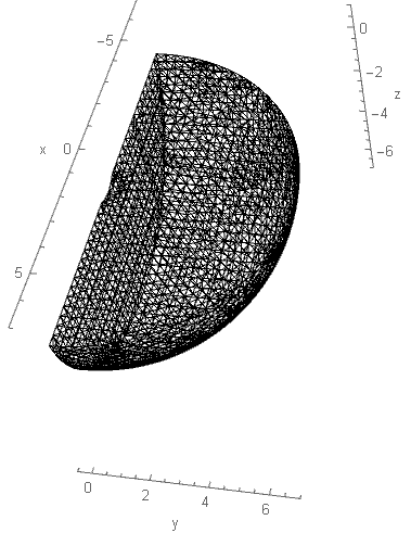
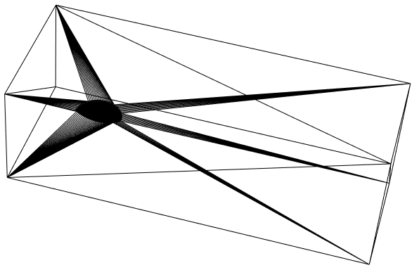
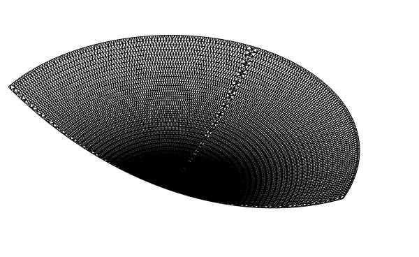
Show[{Graphics3D[{Red, polys[[posXids]]}],
  Graphics3D[{Blue, polys[[negXids]]}]}]
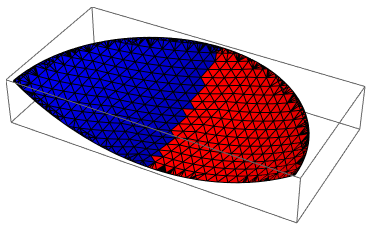
There is a bit of jaggedness at the seam of the left and right-hand sides. Hopefully, the errors will average out. We could have put a seam at the interface with more elaborate model construction. Now, we can estimate the fluxes using the following:
gradT[x_, y_, z_] = {Derivative[1, 0, 0][sol][x, y, z],
   Derivative[0, 1, 0][sol][x, y, z],
   Derivative[0, 0, 1][sol][x, y, z]};
f = NDSolve`FEM`MapThreadDot[(gradT @@@ center3[[#]]), bn3[[#]]] .
    area3[[#]] &;
f[posXids]
f[negXids]
f[posXids~Join~negXids]
(* -0.952311 *)
(* -2.96147 *)
(* -3.91378 *)
These results agree with the OP integral formulation quite well and are significantly faster.
Comparison to another code
When possible, it is always good to compare the Mathematica FEM results with another FEM code. In this case, I will show that the Mathematica results compare favorably with the FEM code COMSOL. First, I will create a SliceContourPlot3D for comparison purposes.
surf = {{x^2 + y^2 + z^2 ==
     1.001^2}, {"XStackedPlanes", {7.5}}, {"YStackedPlanes", {0}}, \
{"ZStackedPlanes", {-0.8}}, {"BackPlanes"}};
SliceContourPlot3D[sol[x, y, z], surf, {x, y, z} ∈ mesh,
 Contours -> 11, PlotPoints -> 100, BoxRatios -> Automatic,
 ColorFunction -> "ThermometerColors", PlotRange -> {-0.001, 1},
 PlotLegends -> Automatic]
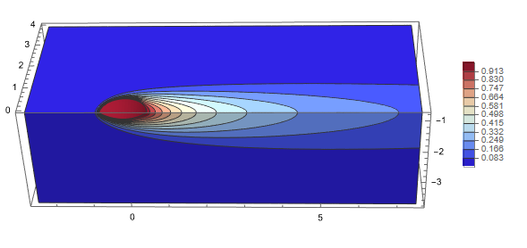
Here is the comparable COMSOL plot:
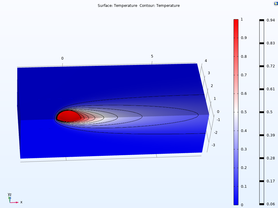
As you can see, the visualizations compare favorably.
We also can see that the integrations of gradT on the left and right hemispherical cap surfaces also agreed to within about 2%
| Application |
Left |
Right |
| Mathematica |
-2.96147 |
-0.95414 |
| COMSOL |
-3.0255 |
-0.952755 |
| %Diff |
2.16226 |
0.0465888 |
Update in response to a comment about low Péclet numbers
The Péclet number is defined by:
$$Pe=\frac{Advective\ Transport\ Rate}{Diffusive\ Transport\ Rate}$$
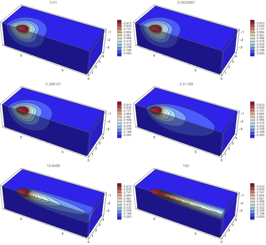
So, as the Péclet number goes down the Advective component becomes less significant indicating that a "wind tunnel" is perhaps not the best model to study this problem. Although you may want to consider modifying the geometry, you can substantially mitigate the effects of low Péclet numbers by changing the default wall conditions to DirichletCondition's. Here is a logarithmic sweep from Pe numbers from 0.01 to 100 (note that this process is slow):
pfun = ParametricNDSolveValue[{D[T[x, y, z], x] ==
     1/P Laplacian[T[x, y, z], {x, y, z}], {DirichletCondition[
      T[x, y, z] == 1., ElementMarker == 3],
     DirichletCondition[T[x, y, z] == 0.,
      Or @@ (ElementMarker == # & /@ {4, 6, 7})]}},
   T, {x, y, z} ∈ mesh, {P}];
surf = {{x^2 + y^2 + z^2 ==
     1.001^2}, {"XStackedPlanes", {7.5}}, {"YStackedPlanes", {0}}, \
{"ZStackedPlanes", {-0.8}}, {"BackPlanes"}};
frames = SliceContourPlot3D[pfun[#][x, y, z],
     surf, {x, y, z} ∈ mesh, Contours -> 11,
     PlotPoints -> 100, BoxRatios -> Automatic,
     ColorFunction -> "ThermometerColors", PlotRange -> {-0.001, 1},
     PlotLegends -> Automatic, PlotLabel -> N@#] & /@ (10^# & /@
     Subdivide[-2, 2, 20]);
ListAnimate[frames]



x^2+y^2+z^2<=4&&x>=0&& y >= 0 && z <= -1 + p, with mesh of 50323 Tetrahedron Element (MaxCellMeasure -> .0001), check solution and then try to expand region. $\endgroup$