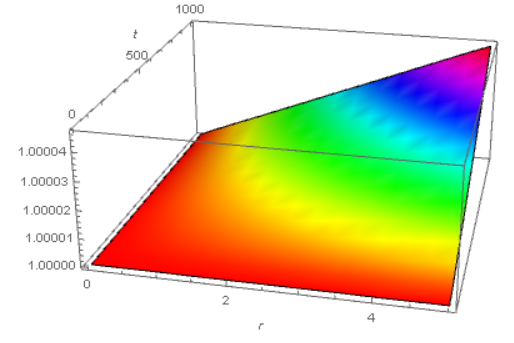
I am currently working on a problem on spheres, in which there is a function Q that is dependent on radius r and time t. I am interested in solving a PDE that gives a picture of evolution of Q over time. I was recommended to use Mathematica since its easier to plot it and so on. The equation is:

where k is a proportionality constant, c is a central value of the sphere, G is the gravitational constant and $\alpha$ depends on $\kappa$ and G. I chose to run with: $\kappa$ = 1; G = $6.67408*10^{-11}$; c = 20; $α = \sqrt{k/(2 \pi G)}$ = 48833.1
My initial code was:
pde = D[Q[r, t], {t, 2}] -
   2*k*c*α*(((Cos[r/α])/(rα)) - ((Sin[
          r/α]/r^2)))*D[Q[r, t], {r, 1}] -
   2*k*c*α*((Sin[r/α]/r)*D[Q[r, t], {r, 2}]) + (2*k*
      c*α*(((Cos[r/α])/(rα)) - ((Sin[r/α]/
           r^2)))*D[
       Q[r, t], {r, 1}])/((cα*(Sin[r/α]/r)) +
      Q[r, t]) - 4*π*G*c*α*(Sin[r/α]/r)*Q[r, t] == 0
i1 := Q[0, t] == 2
i2 := Q[r, 0] == 1

sol = NDSolve[{pde, i1, i2}, Q[r, t], {r, 0, 5}, {t, 0, 10}]
with "test" initial conditions since it wasn't working. After tackling a horde of errors I couldn't figure out where I was going wrong (I assume the problem is due to a variable coefficient) and so I tried simplifying it using variable separation [Q(r,t) = R(r)T(t)] which split it into two parts, the time component:
DSolve[(1/T[t]) D[T[t], {t, 2}] == -L^2, T[t], t]
which works, and the spatial component:
eqn = -2 k c α ((Cos[r/α]/α r) - (Sin[r/α]/r^2)) (1/R[r]) R'[r] -
   2 k c α (Sin[r/α]/r) (1/R[r]) R''[r] +
   2 k ((Cot[r/α]/α) - (1/r)) (1/R[r]) R'[r] -
   4 π G c α (Sin[r/α]/r) == L^2
i3 = R[3] == 5
i4 = R[2] == 2
sol = NDSolve[{eqn, i3, i4}, R[r], r]
which gives an error. The initial conditions here too are guesses.
My questions are, where am I going wrong, and how would I go about plotting Q(r,t)?

