Numerical Integration of KdV Equation by Runge-Kutta 4

Question

I have been asked to reduce the KdV ODE Equation

$d^3/dX^3=(c+6f)df/dX $

to a first order ODE and then solve this ODE by RK4 (Runge-Kutta 4) Numerical Integration.

Analytically, letting c=1 for simplicity, we integrate to get

$f''-3f^2-f=C$

Where $C$ is integration constant. Then Multiply by $f'$ and Integrate to get

$(f')^2/2 -f^3 -f^2/2=Cf +D$

Where $D$ is another integration constant. Now Solve for $f'$ we get

$df/dX=\sqrt(2f^3+f^2+2Cf+2D)$

I have been given initial conditions: $f(0)=-1/2$, $df/dX=0$, and $df^2/dX^2=1/4$

I have been told to:

Use RK4 to integrate numerically the first-order reduction of the ODE from $X = 0$ forward $X_n = n * h, n = 0, 1, . . .N$ and for sufficiently large $X$ (i.e. large $N$). You will need to be plotting $f$ vs $X$ to see if the solution is settling to determine when to stop the integration. Use your judgement as to how small a step size you need to solve this system accurately. If you cannot figure this out from pure thought, experiment with different step sizes and use $δC = |(C(t) − C(t = 0))/C(t = 0)|$ to determine the accuracy. If $δC$ is smaller than $10^{−3}$ for all integration times, then you have acceptable accuracy. Show in a plot your solution for $f(X)$, for $X \in [−20, 20]$.

Here is my Code:

ti = -\[Pi];
tf = \[Pi];
i = 256;
\[CapitalDelta]t = (tf - ti)/i;
X = Range[ti, tf, \[CapitalDelta]t] // N;
F = ConstantArray[0., i + 1];
D1 = ConstantArray[0., i + 1];
D2 = ConstantArray[0., i + 1];
(*Runge Kutta of Order 4*)
F[[1]] = -1/2;
D1[[1]] = 0.;
D2[[1]] = 1/4;

Do[
 k1 = \[CapitalDelta]t*\[Sqrt]Abs[(2 F[[n]]^3 + F[[n]]^2 + 
       2*(D2[[n]] - 3 F[[n]]^2 - F[[n]])* F[[n]] + 
       2*(1/2 D1[[n]]^2 - F[[n]]^3 - 1/2 F[[n]]^2 - D2[[n]] - 
          3 F[[n]]^2 - F[[n]]* F[[n]]))];
 k2 = \[Sqrt]Abs[(2 F[[n]]^3 + F[[n]]^2 + 
       2*(D2[[n]] - 3 F[[n]]^2 - F[[n]])* F[[n]] + 
       2*(1/2 D1[[n]]^2 - F[[n]]^3 - 1/2 F[[n]]^2 - D2[[n]] - 
          3 F[[n]]^2 - F[[n]]* F[[n]]))] + \[CapitalDelta]t*k1/2;
 k3 = \[Sqrt]Abs[(2 F[[n]]^3 + F[[n]]^2 + 
       2*(D2[[n]] - 3 F[[n]]^2 - F[[n]])* F[[n]] + 
       2*(1/2 D1[[n]]^2 - F[[n]]^3 - 1/2 F[[n]]^2 - D2[[n]] - 
          3 F[[n]]^2 - F[[n]]* F[[n]]))] + \[CapitalDelta]t*k2/2;
 k4 = \[Sqrt]Abs[(2 F[[n]]^3 + F[[n]]^2 + 
       2*(D2[[n]] - 3 F[[n]]^2 - F[[n]])* F[[n]] + 
       2*(1/2 D1[[n]]^2 - F[[n]]^3 - 1/2 F[[n]]^2 - D2[[n]] - 
          3 F[[n]]^2 - F[[n]]* F[[n]]))] + \[CapitalDelta]t*k3/2;
 D1[[n + 1]] = D1[[n]] + 1/6*\:f000k1 + 2 k2 + 2 k3 + k4\:f006,
 D2[[n + 1]] = D2[[n]] + 1/6*\:f000k1 + 2 k2 + 2 k3 + k4\:f006,
 F[[n + 1]] = F[[n]] + 1/6*\:f000k1 + 2 k2 + 2 k3 + k4\:f006,
 {n, 1, i}]

So I tried to use 3 vectors with 3 initial values given, and iterate until all the values are filled. but I don't know how to compute the next values of D1 and D2, based on the initial values.

On the other hand, apparently there must be a function with two variable inputs, where it returns a only one F back. I found this online:

Y, T, h = initialize_all(y0, t0, t1, n)
for i in xrange(1, n):
K1 = f(T[i-1], Y[i-1])
tplus = (T[i] + T[i-1]) * .5
K2 = f(tplus, Y[i-1] + .5 * h * K1)
K3 = f(tplus, Y[i-1] + .5 * h * K2)
K4 = f(T[i], Y[i-1] + h * K3)
Y[i] = Y[i-1] + (h / 6.) * (K1 + 2 * K2 + 2 * K3 + K4)
return T, Y

Which is in another language. but clearly my code should follow this pattern. I have tried hard to solve it, but couldn't figure it out. If anyone can help me, I really appreciate their help.

Thanks

Answer 1

We should note first that point $X=0$ is a branching point for the first order equation. Therefore we need to make special step before RK4. Using initial condition we calculate, that $C=D=0$, therefore first order equation looks like $$y'=\pm \sqrt {2 y^3+y^2}$$ Code for RK4 we can organize with Module as follows

rk4[f_, h_, x0_, y0_, n_] := 
 Module[{k1, k2, k3, k4}, T[0] = x0; Y[0] = y0;
  Do[k1 = f[T[i - 1], Y[i - 1]]; T[i] = T[i - 1] + h;
   tplus = (T[i] + T[i - 1])*.5;
   k2 = f[tplus, Y[i - 1] + .5*h*k1];
   k3 = f[tplus, Y[i - 1] + .5*h*k2];
   k4 = f[T[i], Y[i - 1] + h*k3];
   Y[i] = Y[i - 1] + (h/6.)*(k1 + 2*k2 + 2*k3 + k4);, {i, 1, n}]; 
  ysol = Table[{T[i], Y[i]}, {i, 0, n}];
  ysol] 

Now we use it in two branches with first step calculation

fp[x_, y_] := Sqrt[2 y^3 + y^2]; h1 = 10^-6; y1 = -1/2 + h1^2/2 *1/4;

yp = rk4[fp, .1, h1, y1, 200];

fm[x_, y_] := -Sqrt[2 y^3 + y^2]; ym = rk4[fm, -.1, -h1, y1, 200];

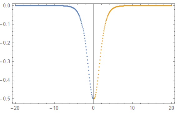
Finally we plot solution

ListPlot[{ym, yp}, PlotRange -> All, Frame -> True]

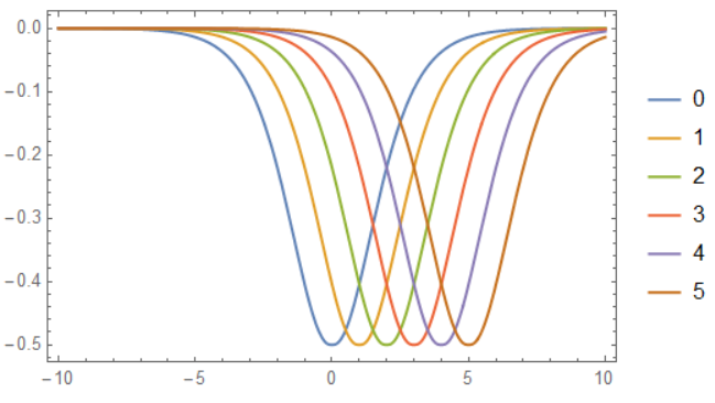
To plot function $y(x-t)$ we can use code

ys = Interpolation[Join[ym, yp]];

Plot[Evaluate[Table[ys[x - t], {t, 0, 5, 1}]], {x, -10, 10}, 
 PlotLegends -> Table[t, {t, 0, 5, 1}], Frame -> True]

To compute parameter $C=y''-3 y^2-y$ for numerical solution we should remember that we solve first order ODE, and therefore we need some interpolation of numerical solution to calculate a second derivative. For this problem we use code

uu[h_, h1_, n_] := 
 Module[{hh = h, nn = n}, fp[x_, y_] := Sqrt[2 y^3 + y^2]; 
  y1 = -1/2 + h1^2/2 *1/4;
  yp = rk4[fp, hh, h1, y1, nn]; fm[x_, y_] := -Sqrt[2 y^3 + y^2]; 
  ym = rk4[fm, -hh, -h1, y1, nn]; un = Join[ym, {{0, -1/2}}, yp]; un] 

Let evaluate uu with input data h=h1=.1;n=200 then we have numerical solution as interpolation function

y = Interpolation[uu[.1, .1, 200], InterpolationOrder -> 4]

With this function we can compute C and plot it in a big and small scale as follows (here ch=C but we can't use letter C as a name since it is the default form for the parameter or constant generated in representing the results of various symbolic computations)

ch = y''[x] - 3 y[x]^2 - y[x];

{LogPlot[Abs[ch], {x, -20, 20}, PlotRange -> All, Frame -> True], 
 LogPlot[Abs[ch], {x, -2, 2}, PlotRange -> All, Frame -> True]}