4
$\begingroup$

I have dielectric functions of materials as lists of value pairs {{x1, y1}, {x2, y2}, ...} and unfortunately some of them are quite long, which is a bother in numerical integration.

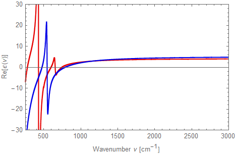
I tried to find a method for "smart under-sampling", meaning that constant regions are undersampled quite strongly while regions with relevant features are sampled more densely (see picture below for an example of plotted data).

After an hour of searching I only found the Downsample function, which only skips values in a fixed step size and has nothing to do what I want to do. I have found options to increase the sample size (e.g., by plotting with a higher interpolation order and extracting the data points), but nothing to reduce it.

Help would be appreciated!

data example

$\endgroup$
2
  • 2
    $\begingroup$ The trapezoidal rule on 10^6 points in an unpacked array takes 0.2–0.3 seconds on my MacBook pro. If the data is packed, performance is about 10 times faster. Example code: With[{x = data[[All, 1]], y = data[[All, 2]]}, With[{dx = Differences@x}, dx . (Most[y] + Rest[y])/2 ]] — would that be accurate & fast enough? $\endgroup$
    – Michael E2
    Jan 8, 2021 at 15:17
  • 2
    $\begingroup$ Fully agree with Michael E2, even 10^6 is not much. Rather, one should worry about the correct asymptotic behavior. $\endgroup$
    – yarchik
    Jan 8, 2021 at 16:02

2 Answers 2

3
$\begingroup$

I suspect you may be worrying too much about the number of points. Numerical integration will be fast even with millions of points, so you are probably fine as you are.

However, you could use the adaptive sampler that is built in to Plot to get what you want. The idea is to construct an interpolating function from your data, then plot it using Plot, which will sample more densely where the rate of change is higher, and more sparsely where the function is smoother. You then extract the resampled points from the Graphics object generated by Plot.

First of all, let's get some fake data to play with:

ClearAll[test]
test[x_] := -((3*(-23 + x/10))/(5*(1/20 + (-23 + x/10)^2)^2)) - 
    (3*(-20 + x/10))/(1/10 + (-20 + x/10)^2)^2 + (25*x)/(50 + x)
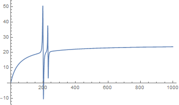
Plot[test[x], {x, 0, 1000}, PlotRange -> All]

fakedata = N@Table[{x, test[x]}, {x, 0, 1000, 1/10}];

shape of the test function, with two derivative-peak spikes

Then interpolate and plot the interpolating function with Plot, using Cases to extract the adaptively-sampled mesh points:

int = Interpolation[fakedata]
resampled = Cases[Plot[int[x], {x, 0, 1000}], Line[pts_] :> Sequence @@ pts, All];

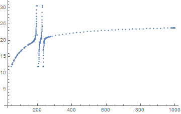
ListPlot[resampled, PlotRange -> All]

resampled data as a ListPlot

As you can see, the "interesting" parts of the curve were sampled more closely, whereas the mostly linear portions were sampled more sparsely.

$\endgroup$
3
$\begingroup$

The problem can be stated as: Given some sequential data, downsample the data according to the rate of change. That means, many samples where the rate of change is high and less samples if it is low.

The idea is to define a function that maps the evenly spaced indices of the data to unevenly spaced indices. Toward this aim we calculate the absolute values of the rate of change of the data: roc. We then invert this values, but because the rate can be zero, we need to add a damping term: 1/(roc+damp). damp will determine how uneven the outcome will be and needs to be adapted to the data. We now have a function that is high where the rate is low and vice versa. If we integrate this function, we get the searched for function that maps the indices unevenly. In the following we have discrete data, therefore we take differences instead of derivatives and accumulate instead of integrate.

We start by defining some test data. Here we choose data over half a period of a sine.

dat = Table[Sin[x], {x, 0, Pi, Pi/100}] // N;
n = Length@dat;

Then we calculate the absolute values of the differences between the data points and invert this to give the inverse rate, using a damping factor of 0.005. Next we accumulate this data. Now, the range of this data is wrong, we need to normalize it to bring it into range 1..n, so that we may use this as indices into the original data.

invrate = 1/(0.005 + Abs@Differences[dat]);
acc = Accumulate[invrate];
newind = Round[n acc/acc[[-1]]];

Now we have everything to downsample the data. As an example we choose a downsampling factor of 5. We create down sampled indices and feed it to newind. Note that we lost one data point when we took the differences, therefore the highest index is: n-1. By this we get the new indices: samplesx, values: samplesy and points: samplesxy that we use for a plot:

samplesx = newind[[Range[1, n - 1, 5]]];
samplesy = dat[[samplesx]];
samplesxy = Table[{i, dat[[i]]}, {i, samplesx}];
ListLinePlot[dat, Epilog -> Point[samplesxy]]
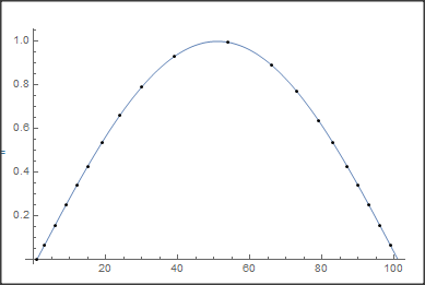
enter image description here

$\endgroup$

Your Answer

By clicking “Post Your Answer”, you agree to our terms of service and acknowledge you have read our privacy policy.

Not the answer you're looking for? Browse other questions tagged or ask your own question.