Optimizing my code for Broyden's method

Question

The following code is my attempt of employing Broyden's method for root finding on the function $f(x,y)=(e^{xy}-y^2-2,\cos(x+y)+\frac{1}{2})$. Where the first matrix is the Jacobian, then it gets updated using an estimate. So $k[l,k]$ computes the first 12 iterations. However, this program is extremely slow and I am not sure why. Could anyone point out why it is so slow and how I could improve it?

k[l_, k_] := Module[{m}, 
  f[{x_, y_}] := {Exp[x y] - y^2 - 2, Cos[x + y] + 1/2};
  h = {Exp[x y] - y^2 - 2, Cos[x + y] + 1/2};
  b = {x, y};
  
  m[0] := {{l}, {k}};
  
  J[0] := D[h, {b}];
  m[n_] := 
   m[n] = N[m[n - 1]] - 
      Inverse[N[J[n - 1]]].N[f[m[n - 1]]] /. {x -> 
       Part[Part[N[m[n - 1]], 1], 1], 
      y -> Part[Part[N[m[n - 1]], 2], 1]};
  J[n_] := 
   J[n] = N[
      J[n - 1]] + ((N[f[m[n]]] - N[f[m[n - 1]]] - 
          N[J[n - 1]].(N[m[n] - m[n - 1]]))/
        Norm[N[m[n] - m[n - 1]]]^2).Transpose[N[m[n]] - N[m[n - 1]]];
  Table[m[a], {a, 1, 12}]]

I would appreciate any input.

EDIT: I found some optimization to my code. I removed the redundant $N$ as per a suggestion in the comments. The optimization I found is to deal with numerical matrices form the get go. The original code did everything for arbitrary $x,y$

k[l_, k_] := Module[{m}, 
  f[{x_, y_}] := {Exp[x y] - y^2 - 2, Cos[x + y] + 1/2};
  h = {Exp[x y] - y^2 - 2, Cos[x + y] + 1/2};
  b = {x, y};
  
  m[0] := N[{{l}, {k}}];
  
  J[0] := 
   N[D[h, {b}]] /. {x -> Part[Part[m[0], 1], 1], 
     y -> Part[Part[m[0], 2], 1]};
  m[n_] := m[n] = m[n - 1] - LinearSolve[J[n - 1], f[m[n - 1]]];
  J[n_] := 
   J[n] = J[
      n - 1] + ((f[m[n]] - f[m[n - 1]] - J[n - 1].(m[n] - m[n - 1]))/
        Norm[m[n] - m[n - 1]]^2).Transpose[m[n] - m[n - 1]];
  Table[m[a], {a, 1, 15}]]
```

Answer 1

The problem with your implementation is the fact that the values of the Jacobian are kept symbolic at every iteration, so their complexity grows exponentially.

For each iteration J[n] should have the value of {x, y} updated from m[n-1]. I am also unravelling the internal definitions of all those functions, removing the unnecessary N calls, and somewhat simplifying the rest of the code:

ClearAll[f, k, J, m]
f[{x_, y_}] = {Exp[x y] - y^2 - 2, Cos[x + y] + 1/2};
J[0] = D[f[{x, y}], {{x, y}}];

(* note the replacement of the values of x and y at the end *)
(* that is critical to obtain numerical values for J at each step *)
(* that was the source of your slowdown *)
J[n_] := J[
    n] = (J[n - 
        1] + ((f@m[n] - f@m[n - 1] - J[n - 1].(m[n] - m[n - 1]))/
         Norm[m[n] - m[n - 1]]^2).(m[n] - m[n - 1])) /. 
    Thread[{x, y} -> m[n - 1]];


m[n_] := m[n] = 
  m[n - 1] - (Inverse[J[n - 1]].f@m[n - 1] /. 
     Thread[{x, y} -> m[n - 1]])

Let's see a trial run:

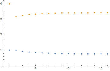
m[0] = N@{1, 4};
results = Table[m[n], {n, 0, 15}]
ListPlot@Transpose@results

{{1., 4.}, {1.00863, 3.17414}, {0.934639, 3.25276}, {0.886161, 3.30122}, {0.852723, 3.33465}, {0.829105, 3.35826}, {0.812153, 3.3752}, {0.799845, 3.38751}, {0.790838, 3.39651}, {0.784208, 3.40314}, {0.779307, 3.40804}, {0.775673, 3.41167}, {0.772972, 3.41437}, {0.770961, 3.41638}, {0.769463, 3.41787}, {0.768345, 3.41899}}

---

The problem still remains that this approach based on matrix inversion at every step is not very efficient, and I am also not sure that it is in the spirit of the method proposed (although I am not familiar with it).

Finally,

FindRoot[f[{x, y}], {x, 1}, {y, 4}]

(* Out: {x -> 0.764945, y -> 3.42385} *)

is built-in and orders of magnitude faster, of course.