4
$\begingroup$

So I know that trigonometric equations show up here very often, but this one is particularly difficult and important to me, so that I was hoping to get some valuable hints from people who know more about equation solving than I do.

I would like to solve the following equations: $$f(x)=\sqrt{a \left(c^2-b \left(c^2+x^2\right)\right)+\left(c^2+x^2\right) \left((b-1) c^2+b x^2-e\right)}/\sqrt{-a+c^2+x^2}$$ $$x \cot (x\,d)=-f(x) \cot (f(x)\,d)$$ or in code form:

f[x_] = Sqrt[(c^2 + x^2) ((-1 + b) c^2 - e + b x^2) + a (c^2 - b (c^2 + x^2))]/Sqrt[-a + c^2 + x^2]
x Cot[x d] == -f[x] Cot[f[x] d]

where a, b, c, d and e are arbitrary constants which can become very small (~1e-30) or very large (~1e30).

I tried FindRoot[], which works very well for constants of the order of ~1e0 to ~1e1 but breaks down for extremely big or small numbers. In particular, I find multiple duplicates, and solutions that do not actually solve the equation above. To make the code more stable, I squared both sides of the second equation (the roots don't change), as FindRoot[] converges quicker for positive functions. Furthermore, looking at the graphs for the RHS and LHS of the second equation, one can see that the cotangent has a $\pi$-periodicity which helps determining the range in which FindRoot is supposed to look for solutions:

FR[n_] := FindRoot[(x Cot[x d])^2 == (-f[x] Cot[f[x] d])^2, {x,Pi*n/4 - 0.001, Pi*(n + 1)/4 - 0.001}]
sol = Map[FR, Range[0, 50, 1]];
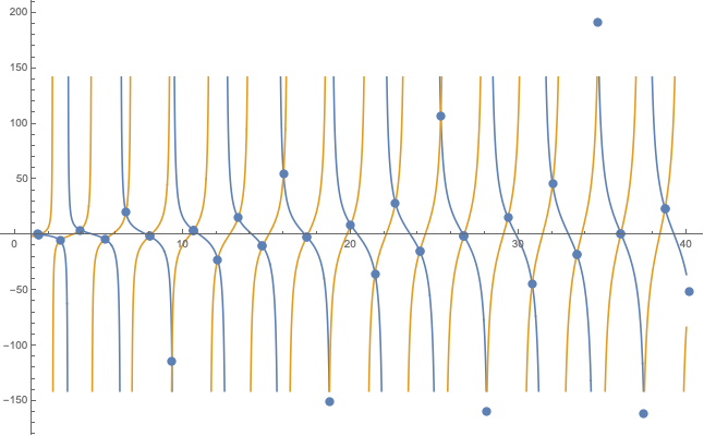
p1 = Plot[{x Cot[x d],-f[x] Cot[f[x] d]}, {x, 1, 40}];
p2 = ListPlot[Transpose[{x /. sol, x Cot[x d] /. sol}]];
Show[p1, p2, PlotRange -> Automatic]

enter image description here

Unfortunately, this does not work so smoothly for extreme values such as

a = 10^14; b = 10^(-18); c = 10^6; d = 10; e = 10^(-18);

Could someone tell me how I can make this code more stable or suggest an alternative way of solving this equation?

$\endgroup$
13
  • $\begingroup$ I would suggest to use rational values 1/1000 instead of 0.001 and explicitly set WorkingPrecision for FindRoot to value larger that MachinePrecision, i.e WorkingPrecision->17. If that will not help, please provide explicit values for which you obtain parasite solutions. $\endgroup$
    – Acus
    Commented Oct 30, 2020 at 14:00
  • $\begingroup$ Working with a nonlinear trigonometric equation it is resonable to take into acount a few hints e.g. listed in this answer: Solve symbolically a transcendental trigonometric equation and plot its solutions $\endgroup$
    – Artes
    Commented Oct 30, 2020 at 14:02
  • $\begingroup$ It might help to know a little more about your ultimate goal. You mention periodicity, but the periodicity of the two expressions is not equal so only special cases where the periods are commensurable will yield a finite number of unique solutions. You're obviously not looking for an analytical expression. How many numerical solutions do you need? $\endgroup$
    – N.J.Evans
    Commented Oct 30, 2020 at 14:06
  • 1
    $\begingroup$ @user18792 I updated the question with some explicit values for which I would like to find a solution. Setting the WorkingPrecision did not give me any useful results after Mathematica ran for 45 min so I aborted the computation. $\endgroup$
    – xabdax
    Commented Oct 30, 2020 at 14:58
  • 2
    $\begingroup$ I want to say, that once your set parameters values, then before calling FindRoot your have to check that f[x] yields real values for starting search interval. One way to get conditions for them is to use Reduce in the above way (both for numerator and denominator) $\endgroup$
    – Acus
    Commented Oct 30, 2020 at 16:47

1 Answer 1

3
$\begingroup$

I am expanding on my comment. You want to find $x,y$ such that:

$$ X\cot X + Y\cot Y =0, \ X=d\times x,\ Y=d\times y, \quad \text{and}\quad Y=f(X).$$

$d$ can be seen as a scaling parameter, for simplicity I write the equations here with $d=1$. The problem becomes:

$$x\cot x + y \cot y=0\quad\text{and}\quad y=f(x)$$

These are two equations, that individually are not too complicated. We are going to take advantage of this uncoupling to simplify the numerical resolution.

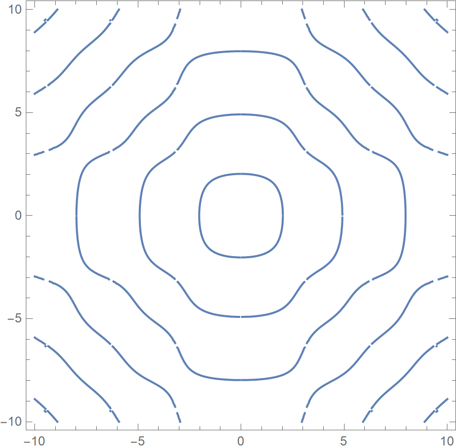
A side node: the first equation can be visualized with ContourPlot:

 ContourPlot[{x*Cot[x] + y*Cot[y] == 0}, {x, -10, 10}, {y, -10, 10}, PlotPoints -> 25]

enter image description here

It is a family of curves that must be not too difficult to find by continuation. Of course the obvious symmetries $y=x$, $x=0$ and $y=0$ should be considered to reduce the computational cost by 8. You are looking for the intersection of these curves with $f(x)=y$. End of side note

Now, you can see that $f^2$ is quite a simple function:

f[x_] = Sqrt[(c^2 + x^2)((-1 + b) c^2 - e + b x^2)+a(c^2 - b (c^2 + x^2))]/Sqrt[-a + c^2 + x^2];
f[x]^2 // FullSimplify
(* (-1 + b) c^2 + b x^2 + e (-1 - a/(-a + c^2 + x^2)) *)

This is an indication that Mathematica can find analytical solutions to $f(x)=y$:

xsol = x /. Solve[f[x] == y, x] // Last // Simplify
(* Sqrt[(a b + c^2 - 2 b c^2 + e + y^2 + Sqrt[ a^2 b^2 - 2 a b (c^2 - e + y^2) + (c^2 + e + y^2)^2])/b]/Sqrt[2] *)

Not that Solve returned 4 solutions, I just kept the last one since it corresponded the real and positive value with the set of parameter I played with.

We can plug that back into the $\cot$ equation:

toroot[y_] = Simplify[xsol*Cot[xsol*d] + f[xsol]*Cot[f[xsol]*d], 
                    Assumptions -> a > 0 && b > 0 && c > 0 && d > 0 && e > 0 && y > 0]

enter image description here

and you end up with a nice, not too complicated function, to solve.


Example 1

a = b = c = d = e = 1;
NSolve[{toroot[y], 0 <= y <= 10}, y]
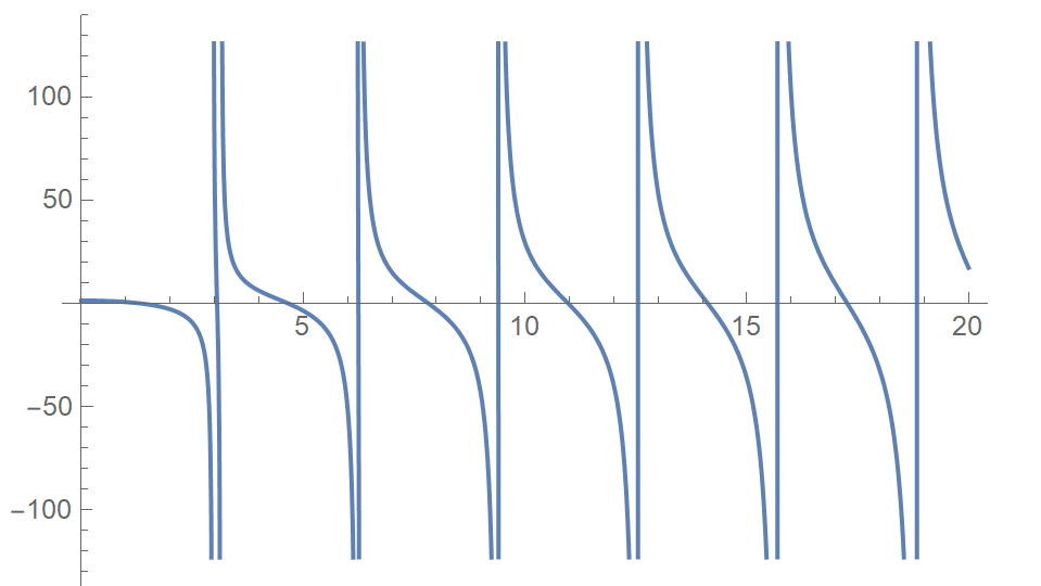
Plot[toroot[y], {y, 0, 20}]
(* {{y -> 1.32709}, {y -> 3.05686}, {y -> 4.65635}, {y -> 6.24267}, {y ->
7.82151}, {y -> 9.39803}} *)

enter image description here

That gives you the $y$ values. Compute the $x$ using: xsol /. y -> ...


Example 2

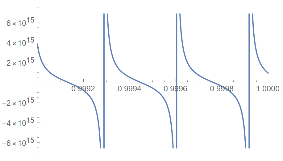
Here, due to the large ratio between a and b, we need to drastically increase WorkingPrecision. Also, toroot is highly oscillatory so I restrict the domain to $[0.999, 1]$

a = 10^14; b = 10^(-18); c = 10^6; d = 10; e = 10^(-18);
NSolve[{toroot[y], 0.999 <= y <= 1.}, y, WorkingPrecision -> 100]
Plot[toroot[y], {y, 0.999, 1.}, WorkingPrecision -> 100]
(* {{y -> 0.9991315326455330769499064220676412494508654045149413025951079\
    640308969038148391768838923514208798058}, 
    {y -> 0.99944591552386175181844643447881974202302427515487185004566648939\
     95674269572854160671851261222602081}} *)

We can check that it is an actual solution:

 xtmp = xsol /. First[NSolve[{toroot[y], 0.999 <= y <= 1.}, y, WorkingPrecision -> 100]]
 xtmp*Cot[d*xtmp] + f[xtmp]*Cot[d*f@xtmp]
 (* 0.*10^-82 *)

enter image description here

$\endgroup$
3
  • $\begingroup$ It seems like NSolve does a good job finding the roots in Example 1, but Example 2 is not very convincing. If you use the results to find the x values and then insert these x values into xsol*Cot[xsol*d] + f[xsol]*Cot[f[xsol]*d] you would expect this expression to become zero. That is not quite what is happening, so I assume that NSolve fails for highly oscillatory functions. $\endgroup$
    – xabdax
    Commented Oct 31, 2020 at 14:41
  • $\begingroup$ @xabdax Most likely due to the huge values involved. Have you tried increasing WorkingPrecision? $\endgroup$
    – anderstood
    Commented Oct 31, 2020 at 15:06
  • 3
    $\begingroup$ Yes, that helps! Great answer by the way! $\endgroup$
    – xabdax
    Commented Oct 31, 2020 at 15:16

Your Answer

By clicking “Post Your Answer”, you agree to our terms of service and acknowledge you have read our privacy policy.

Not the answer you're looking for? Browse other questions tagged or ask your own question.