4
$\begingroup$

I am plotting a vector plot that should represent trajectories through a space of values.

When the trajectories hit one of the boundaries (the values 0 or 1 on each axis), the trajectories are not supposed to be able to go any further. So at that point, the trajectories should evolve along the edge.

I am wondering how to produce this in a plot.

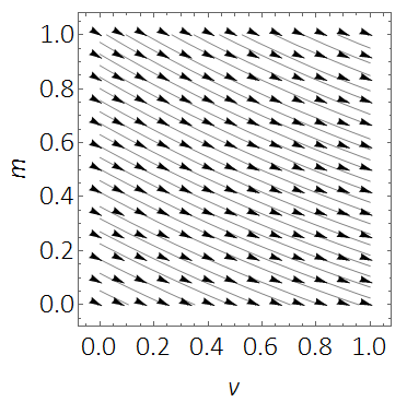
Currently, the vector plot doesn't 'know' that the trajectories cannot go above 1 or below 0 on each axis, so they aren't producing the trajectories I need along the edge. I'd be grateful to anyone who knows how to solve this.

x = 2;
y = 1;
k = 3;


Plota = VectorPlot[{
   
   (1/2 (x k - 
       2 y - (x - y) (-1 + 
          k) mbar + ((x^2) k - (x*y) (-1 + k) x) x) (-1 + x)),
   
   (1/2 (-1 + k) (y + x (-1 + vbar) - x vbar + 
       y (x (-1 + vbar) - y vbar)))
   
   },
  
  {vbar, 0, 1}, {mbar, 0, 1},
  
  VectorStyle -> {"Arrow", Black, Opacity[1]},
  VectorScale -> {0.01, 6, None},
  VectorPoints -> 13,
  
  StreamPoints -> 200,
  StreamScale -> {Full, All, 0.05},
  StreamStyle -> {"Line", Black, Opacity[0.5]},
  
  FrameLabel -> {"v", "m"},
LabelStyle -> Directive[ 25, Black, FontFamily -> "Calibri Light"]]

That produces this:

enter image description here

$\endgroup$
2
  • $\begingroup$ So the expected outcome is an additional arrow that moves anti-clockwise along the frame? $\endgroup$
    – C. E.
    Commented Jul 2, 2020 at 16:05
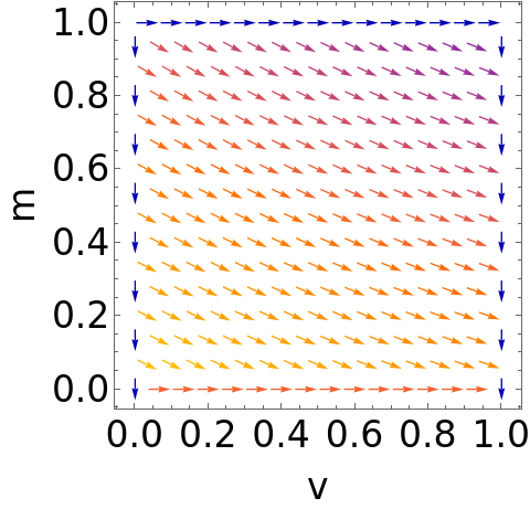
  • $\begingroup$ In this particular case, it would be going horizontally right when m = 0, and vertically down for v = 1. When v = 1, v isn't supposed to be growing any further (since there is no value above 1), but m is still falling. I guess I could just manually plot that, but was wondering if there is a neater way. $\endgroup$
    – Sprog
    Commented Jul 2, 2020 at 16:08

1 Answer 1

3
$\begingroup$

Here's a way to use VectorPlot for this purpose:

x = 2;
y = 1;
k = 3;

v[vbar_, mbar_] := {
  (1/2 (x k - 2 y - (x - y) (-1 + k) mbar + ((x^2) k - (x*y) (-1 + k) x) x) (-1 + x)),
  (1/2 (-1 + k) (y + x (-1 + vbar) - x vbar + y (x (-1 + vbar) - y vbar)))
  }
vRestricted[vbar_, mbar_] := Which[
  vbar > 0.98 || vbar < 0.02, Projection[v[vbar, mbar], {0, 1}],
  mbar > 0.98 || mbar < 0.02, Projection[v[vbar, mbar], {1, 0}],
  True, v[vbar, mbar]
  ]

VectorPlot[
  vRestricted[vbar, mbar],
  {vbar, 0, 1},
  {mbar, 0, 1},
  FrameLabel -> {"v", "m"},
  LabelStyle -> Directive[25, Black, FontFamily -> "Calibri Light"]
  ]

Output

A caveat is that this is very sensitive to the arguments that you supply to VectorPlot. If you sample the space differently, you may miss the vertical and horizontal arrows, get multiple rows of them, or get arrows on the border that aren't perfectly aligned.

A more reliable way of doing this would be to draw the arrows along the border manually, for example using the Epilog option.

One way to take this idea further if you want to have a smooth transition from the outer behavior and the inner behavior, would be to linearly interpolate v and the projection depending on how close to the border the position is.

$\endgroup$
1
  • $\begingroup$ Thank you! This is very clear. $\endgroup$
    – Sprog
    Commented Jul 3, 2020 at 7:43

Your Answer

By clicking “Post Your Answer”, you agree to our terms of service and acknowledge you have read our privacy policy.

Not the answer you're looking for? Browse other questions tagged or ask your own question.