Making a table excluding a region; conditional iteration

Question

I just would like to create the table with the following condition; selecting the points outside a circle

Norm[{x, y}] > 0.5

I used

dataee = 
  Flatten[
    Table[
      {x, y, Phi[x, y] && Norm[{x, y}] > 0.51}, 
      {x, 0.01, 1.3, 0.05}, {y, 0.01, 1.3, 0.05}],
    1];

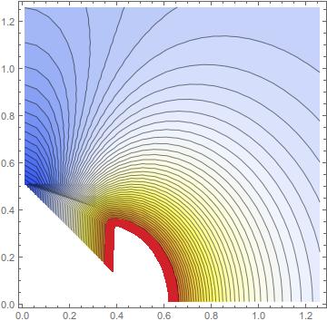
but ListContourPlot still shows the contours inside that circle (the excluded region) which makes the plot useless.

What is the proper way to include this condition while iterating over the loops?

In case one needs the function:

zc = -1.8;
zp = 0.9;
qe = 1.0;
a = 0.22;
σ = 0.5;
κ = 5.0/σ;
ϵ = 80.0;

Phi[x_, y_] := 
  (qe^2/ϵ) (Exp[-κ Norm[{x, y}]]/Norm[{x, y}]) (Exp[κ σ]/((1 + κ σ)))^2 
    ((zc^2 + 2 zc zp 
      (Sum[(a/σ)^i (2 i + 1) LegendreP[i, Cos[ArcTan[y, x]]] Boole[i/2 ∈ Integers], {i, 1, 200}])) + 
     (zc zp + 
        2 zp^2 (Sum[(a/σ)^i (2 i + 1) LegendreP[i, Cos[ArcTan[y + a, x]]] Boole[i/2 ∈ Integers], {i, 1, 200}])) 
     (Exp[-κ Norm[{x, y}] ((Norm[{x, y + a}]/Norm[{x, y}])) - 1] / 
        (Norm[{x, y + a}]/Norm[{x, y}])) + 
     (zc zp + 
        2 zp^2 
          (Sum[(a/σ)^i (2 i + 1) LegendreP[i, Cos[ArcTan[y - a, x]]] Boole[i/2 ∈ Integers], {i, 1, 200}])) 
     (Exp[-κ Norm[{x, y}] ((Norm[{x, y - a}]/Norm[{x, y}])) - 1] / 
       (Norm[{x, y - a}]/Norm[{x, y}])));

This is the plot

Edit:

I can do something similar to the below lines which excludes the points inside the above mentioned circle, but I cannot plot the data. I do not know what is the problem, Flatten does not work and the ListContourPlot output is a blank plot. Here is the method; same function and parameters, instead the output is written into a file.

For[x = 0.01 , x <= 1.3, x += 0.1,
 For[y = 0.01 , y <= 1.3, y += 0.1,
If[Norm[{x, y}] > 0.5, { x, y, Phi[x, y]} >>> "EE.dat"];  ]]

Answer 1

    Clear["`*"];
    zc = -1.8;
    zp = 0.9;
    qe = 1.0;
    a = 0.22;
    σ = 0.5;
    κ = 5.0/σ;
    ϵ = 80.0;
    
    Phi[x_?NumericQ, 
      y_?NumericQ] := (qe^2/ϵ) (Exp[-κ Norm[{x, y}]]/
        Norm[{x, 
          y}]) (Exp[κ σ]/((1 + κ σ)))^2 \
    ((zc^2 + 2 zc zp (Total@
             Table[(a/σ)^i (2 i + 1) LegendreP[i, 
                Cos[ArcTan[y, x]]], {i, 2, 200, 2}])) + (zc zp + 
           2 zp^2 (Total@
              Table[(a/σ)^i (2 i + 1) LegendreP[i, 
                 Cos[ArcTan[y + a, x]]], {i, 2, 200, 
                2}])) (Exp[-κ Norm[{x, 
                y}] ((Norm[{x, y + a}]/Norm[{x, y}])) - 
             1]/(Norm[{x, y + a}]/Norm[{x, y}])) + (zc zp + 
           2 zp^2 (Total@
              Table[(a/σ)^i (2 i + 1) LegendreP[i, 
                 Cos[ArcTan[y - a, x]]], {i, 2, 200, 
                2}])) (Exp[-κ Norm[{x, 
                y}] ((Norm[{x, y - a}]/Norm[{x, y}])) - 
             1]/(Norm[{x, y - a}]/Norm[{x, y}])));
 data = 
     Table[{x, y, Phi[x, y]}, {x, 0.01, 1.3, 0.02}, {y, 0.01, 1.3, 0.02}];
    newdata = 
      Cases[{a_Real, b_Real, c_Real} /; Norm[{a, b}] > 0.5] /@ data;
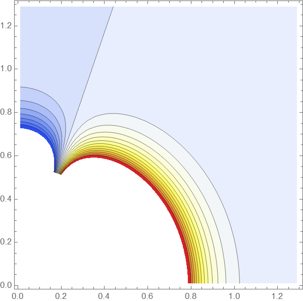
    ListContourPlot[Flatten[newdata, 1], 
     RegionFunction -> (Norm[{#1, #2}] > 0.55 &), Contours -> 20, 
     ColorFunction -> "TemperatureMap"]

Clear["`*"];
zc = -1.8;
zp = 0.9;
qe = 1.0;
a = 0.22;
\[Sigma] = 0.5;
\[Kappa] = 5.0/\[Sigma];
\[Epsilon] = 80.0;
Phi[x_?NumericQ, 
   y_?NumericQ] := (qe^2/\[Epsilon]) (Exp[-\[Kappa] Norm[{x, y}]]/
     Norm[{x, 
       y}]) (Exp[\[Kappa] \[Sigma]]/((1 + \[Kappa] \[Sigma])))^2 \
((zc^2 + 2 zc zp (Total@
          Table[(a/\[Sigma])^i (2 i + 1) LegendreP[i, 
             Cos[ArcTan[y, x]]], {i, 2, 200, 2}])) + (zc zp + 
        2 zp^2 (Total@
           Table[(a/\[Sigma])^i (2 i + 1) LegendreP[i, 
              Cos[ArcTan[y + a, x]]], {i, 2, 200, 
             2}])) (Exp[-\[Kappa] Norm[{x, 
             y}] ((Norm[{x, y + a}]/Norm[{x, y}])) - 
          1]/(Norm[{x, y + a}]/Norm[{x, y}])) + (zc zp + 
        2 zp^2 (Total@
           Table[(a/\[Sigma])^i (2 i + 1) LegendreP[i, 
              Cos[ArcTan[y - a, x]]], {i, 2, 200, 
             2}])) (Exp[-\[Kappa] Norm[{x, 
             y}] ((Norm[{x, y - a}]/Norm[{x, y}])) - 
          1]/(Norm[{x, y - a}]/Norm[{x, y}])));
data = Table[{x, y, Phi[x, y]}, {x, 0.01, 1.3, 0.02}, {y, 0.01, 1.3, 
    0.02}];
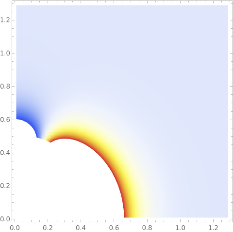
ListDensityPlot[Flatten[data, 1], ColorFunction -> "TemperatureMap", 
 RegionFunction -> Function[{x, y}, Norm[{x, y}] > 0.51]]

Answer 2

First, I simplified function Phi to speed-up computation:

zc = -1.8;
zp = 0.9;
qe = 1.0;
a = 0.22;
\[Sigma] = 0.5;
\[Kappa] = 5.0/\[Sigma];
\[Epsilon] = 80.0;

Phi[x_?NumericQ, y_?NumericQ] := (qe^2/\[Epsilon]) (Exp[-\[Kappa] Norm[{x, y}]]/
 Norm[{x, y}]) (Exp[\[Kappa] \[Sigma]]/((1 + \[Kappa] \[Sigma])))^2 \
((zc^2 + 2 zc zp (Total@
      Table[(a/\[Sigma])^i (2 i + 1) LegendreP[i, 
         Cos[ArcTan[y, x]]], {i, 2, 200, 2}])) + (zc zp + 
    2 zp^2 (Total@
       Table[(a/\[Sigma])^i (2 i + 1) LegendreP[i, 
          Cos[ArcTan[y + a, x]]], {i, 2, 200, 2}])) (Exp[-\[Kappa] Norm[{x, 
         y}] ((Norm[{x, y + a}]/Norm[{x, y}])) - 
      1]/(Norm[{x, y + a}]/Norm[{x, y}])) + (zc zp + 
    2 zp^2 (Total@
       Table[(a/\[Sigma])^i (2 i + 1) LegendreP[i, 
          Cos[ArcTan[y - a, x]]], {i, 2, 200, 2}])) (Exp[-\[Kappa] Norm[{x, 
         y}] ((Norm[{x, y - a}]/Norm[{x, y}])) - 
      1]/(Norm[{x, y - a}]/Norm[{x, y}])));

Now we can plot:

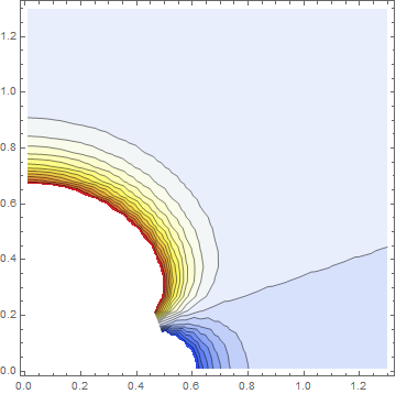
ListContourPlot[Table[Phi[x, y], {x, 0.01, 1.3, 0.05}, {y, 0.01, 1.3, 0.05}], 
RegionFunction -> (Norm[{#1, #2}] > 0.51 &), 
DataRange -> {{0.01, 1.3}, {0.01, 1.3}}, Contours -> 20,
ColorFunction -> "TemperatureMap"]