5
$\begingroup$

Preparations

Mathematica 11.3, Windows.

Let us say I have a rectangular region with 10 little holes inside. Their coordinates are given by positionList. The resulting region mr is made through RegionDifference and RegionUnion of disks and rectangles:

Needs["NDSolve`FEM`"]

radius = 0.1;
Louter = 2;
OuterRegion = Rectangle[{-L/2, -L/2}, {L/2, L/2}] /. L -> Louter;

positionList = {{0.706`, -0.14`}, {0.389`, 0.593`}, {-0.278`, 
    0.429`}, {0.254`, 
    0.844`}, {-0.46`, -0.367`}, {0.737`, -0.759`}, {-0.07`, -0.664`}, \
{-0.469`, 0.626`}, {-0.755`, -0.509`}, {-0.455`, -0.015`}};
diskRegions = Disk[#, radius] & /@ positionList;
mr = RegionDifference[OuterRegion, RegionUnion@diskRegions];

LP = ListPlot[positionList -> Table[k, {k, 1, Length@positionList}]];
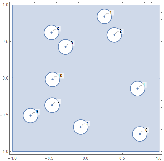
RP = Show[mr // RegionPlot, LP, ImageSize -> 400]

enter image description here

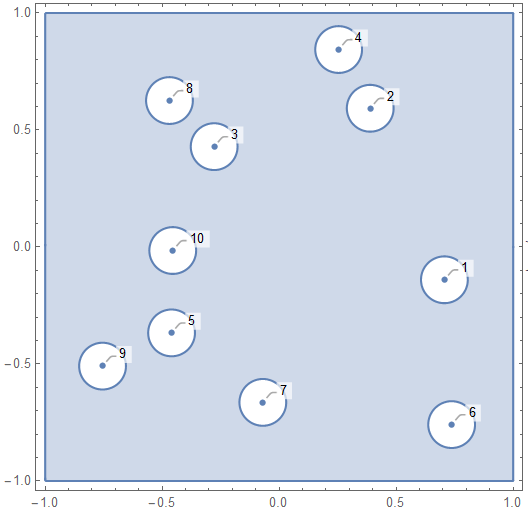
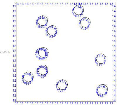
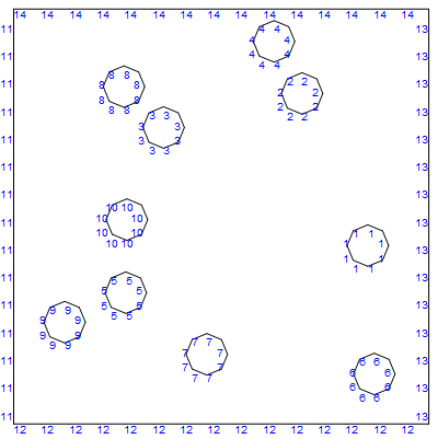
The labels of the disks show the order in which they appear in positionList. Ultimately I want a FEM mesh where I can apply specific boundary conditions on disk 1, disk 2, disk 3 etc. First, I make a boundary mesh:

bmesh = ToBoundaryMesh[RegionBoundary@mr, 
   "RegionHoles" -> positionList, "BoundaryGroupingThreshold" -> 0, 
   AccuracyGoal -> 1];
Show[bmesh["Wireframe"["MeshElementMarkerStyle" -> Blue]], 
 ImageSize -> 400]

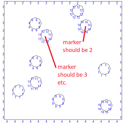
enter image description here

Problem

As you can see, the Region Markers are scrambled! In the boundary mesh, the hole corresponding to disk 2 (in the blue plot above) actually has marker 14. Hole 3 has marker 13, and so on.

I want the markers of the boundary mesh to be consistent with the disk numbers, here going from 1 to 10. The markers on the walls should have numbers 11-14.

A manual solution

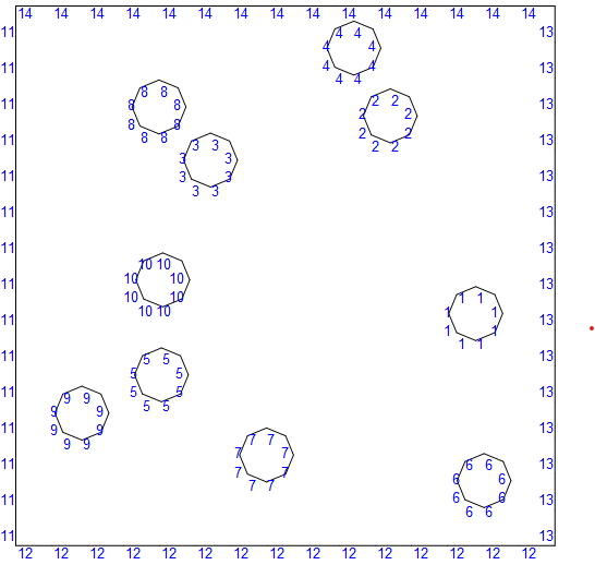
I have solved this problem with a BoundaryMarkerFunction, writing a condition manually for each disk and each of the walls:

boundaryMarkerFunction = 
  Compile[{{boundaryElementCoords, _Real, 
     3}, {pointMarkres, _Integer, 2}},
   Module[{pt1 = #[[1]], pt2 = #[[2]]},
      Which[

       (pt1[[1]] - positionList[[1]][[1]])^2 + (pt1[[2]] - 
            positionList[[1]][[2]])^2 < 
         1.1 radius^2 && (pt2[[1]] - 
            positionList[[1]][[1]])^2 + (pt2[[2]] - 
            positionList[[1]][[2]])^2 < 1.1 radius^2 , 1,
       (pt1[[1]] - positionList[[2]][[1]])^2 + (pt1[[2]] - 
            positionList[[2]][[2]])^2 < 
         1.1 radius^2 && (pt2[[1]] - 
            positionList[[2]][[1]])^2 + (pt2[[2]] - 
            positionList[[2]][[2]])^2 < 1.1 radius^2 , 2,
       (pt1[[1]] - positionList[[3]][[1]])^2 + (pt1[[2]] - 
            positionList[[3]][[2]])^2 < 
         1.1 radius^2 && (pt2[[1]] - 
            positionList[[3]][[1]])^2 + (pt2[[2]] - 
            positionList[[3]][[2]])^2 < 1.1 radius^2 , 3,
       (pt1[[1]] - positionList[[4]][[1]])^2 + (pt1[[2]] - 
            positionList[[4]][[2]])^2 < 
         1.1 radius^2 && (pt2[[1]] - 
            positionList[[4]][[1]])^2 + (pt2[[2]] - 
            positionList[[4]][[2]])^2 < 1.1 radius^2 , 4,
       (pt1[[1]] - positionList[[5]][[1]])^2 + (pt1[[2]] - 
            positionList[[5]][[2]])^2 < 
         1.1 radius^2 && (pt2[[1]] - 
            positionList[[5]][[1]])^2 + (pt2[[2]] - 
            positionList[[5]][[2]])^2 < 1.1 radius^2 , 5,
       (pt1[[1]] - positionList[[6]][[1]])^2 + (pt1[[2]] - 
            positionList[[6]][[2]])^2 < 
         1.1 radius^2 && (pt2[[1]] - 
            positionList[[6]][[1]])^2 + (pt2[[2]] - 
            positionList[[6]][[2]])^2 < 1.1 radius^2 , 6,
       (pt1[[1]] - positionList[[7]][[1]])^2 + (pt1[[2]] - 
            positionList[[7]][[2]])^2 < 
         1.1 radius^2 && (pt2[[1]] - 
            positionList[[7]][[1]])^2 + (pt2[[2]] - 
            positionList[[7]][[2]])^2 < 1.1 radius^2 , 7,
       (pt1[[1]] - positionList[[8]][[1]])^2 + (pt1[[2]] - 
            positionList[[8]][[2]])^2 < 
         1.1 radius^2 && (pt2[[1]] - 
            positionList[[8]][[1]])^2 + (pt2[[2]] - 
            positionList[[8]][[2]])^2 < 1.1 radius^2 , 8,
       (pt1[[1]] - positionList[[9]][[1]])^2 + (pt1[[2]] - 
            positionList[[9]][[2]])^2 < 
         1.1 radius^2 && (pt2[[1]] - 
            positionList[[9]][[1]])^2 + (pt2[[2]] - 
            positionList[[9]][[2]])^2 < 1.1 radius^2 , 9,
       (pt1[[1]] - positionList[[10]][[1]])^2 + (pt1[[2]] - 
            positionList[[10]][[2]])^2 < 
         1.1 radius^2 && (pt2[[1]] - 
            positionList[[10]][[1]])^2 + (pt2[[2]] - 
            positionList[[10]][[2]])^2 < 1.1 radius^2 , 10,
       pt1[[1]] < -0.99 && pt2[[1]] < -0.99, 11, (* left wall *)
       pt1[[2]] < -0.99 && pt2[[2]] < -0.99, 12, (* bottom wall *)
       pt1[[1]] > 0.99 && pt2[[1]] > 0.99, 13, (* right wall *)
       pt1[[2]] > 0.99 && pt2[[2]] > 0.99, 14, (* top wall *)

       True, 4 ]] & /@ boundaryElementCoords];

bmesh = ToBoundaryMesh[RegionBoundary@mr, 
   "RegionHoles" -> positionList, "BoundaryGroupingThreshold" -> 0, 
   AccuracyGoal -> 2, 
   "BoundaryMarkerFunction" -> boundaryMarkerFunction];
{Show[bmesh["Wireframe"["MeshElementMarkerStyle" -> Blue]], 
  ImageSize -> 400], RP}

enter image description here enter image description here

An automatic solution?

Could this be automated, so I can vary the number of disks? I would have happily replaced the Which construct by some Table, but I am not sure what kind of arguments this mysterious boundaryMarkerFunction takes. For instance, I tried

boundaryMarkerFunction[bmesh["BoundaryElements"], 
 bmesh["Coordinates"]]

which fails because boundaryElementCoords is supposed to be 3D.

Please help me find an automatic solution to label the boundary elements in my desired order.

Just for fun

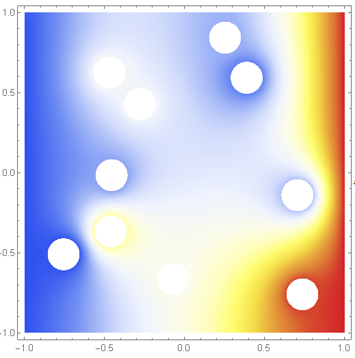
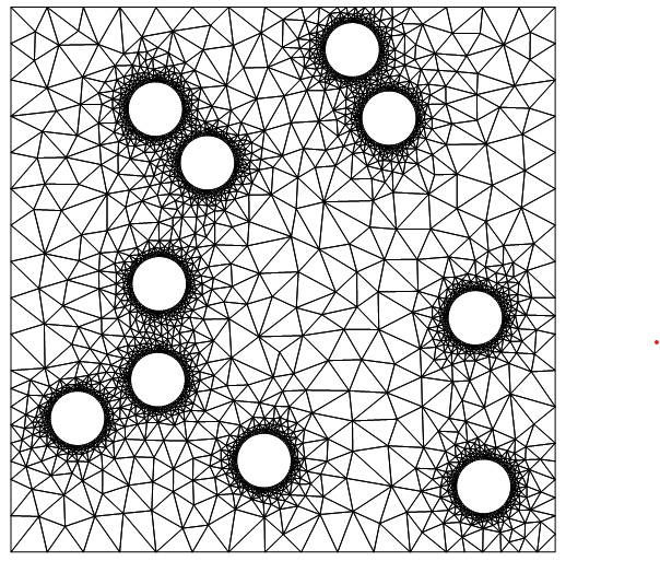
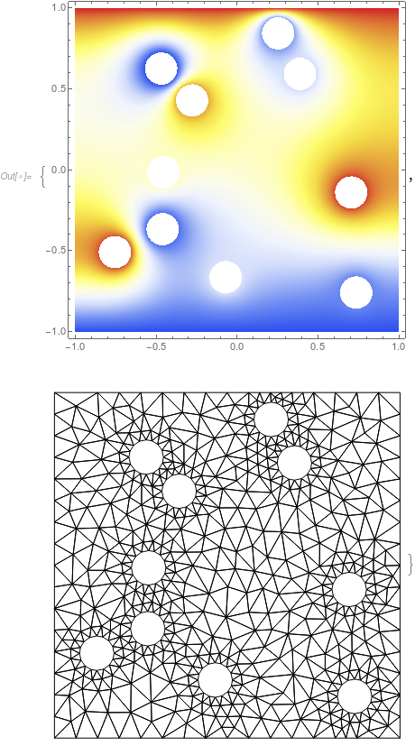
This allows us to use ElementMarker with NDSolve, specifying precise individual boundary conditions on the disks. For instance, here is the heat equation with a different DirichletCondition on each disk:

bmesh = ToBoundaryMesh[RegionBoundary@mr, 
   "RegionHoles" -> positionList, "BoundaryGroupingThreshold" -> 0, 
   AccuracyGoal -> 4, 
   "BoundaryMarkerFunction" -> boundaryMarkerFunction];
mesh = ToElementMesh[bmesh];

boundaryMarkerList = Table[k, {k, 1, Length@positionList}];

op = - Laplacian[u[x, y], {x, y}] + 0.1 u[x, y];
BCedges = {DirichletCondition[u[x, y] == 0, ElementMarker == 11], 
   DirichletCondition[u[x, y] == 1, ElementMarker == 13]};
BCcircles = 
  Table[DirichletCondition[u[x, y] == RandomReal[{0, 1}], 
    ElementMarker == k], {k, 1, Length@positionList}];
BC = Join[BCedges, BCcircles];
ufun = NDSolveValue[{op == 0, BC}, u, {x, y} \[Element] mesh]

{
 DensityPlot[ufun[x, y], {x, y} \[Element] mesh, 
  ColorFunction -> "Temperature", AspectRatio -> Automatic, 
  PlotPoints -> 100, PlotRange -> All, ImageSize -> 400],
 Show[mesh["Wireframe"], ImageSize -> 400]
 }

enter image description here enter image description here

$\endgroup$
3
  • $\begingroup$ If you share the answer to this question I will help you here. $\endgroup$
    – user21
    Commented Jul 22, 2019 at 5:23
  • $\begingroup$ @user21 That question has torus geometry part, where reducing Pe number and increasing mesh precision clearly helped (see edits 1 & 2 in my question). The discrepancy on imported 3D geometry (edit 3) is a more difficult problem. I ended up spending a lot of time simulating this in Comsol, carefully checking flux conservation, resulting in two papers, here and here. I describe my thoughts in more detail in a new EDIT 4 in that question. I hope this works for you. $\endgroup$ Commented Jul 22, 2019 at 11:42
  • $\begingroup$ Thanks for the update. $\endgroup$
    – user21
    Commented Jul 22, 2019 at 12:46

2 Answers 2

6
$\begingroup$

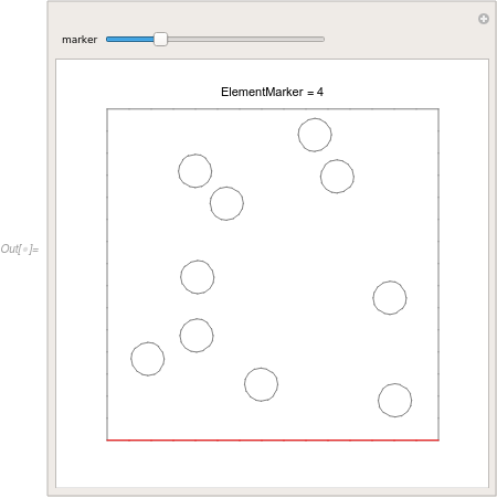
When ElementMarker are attributed automatically there is no way that they would fit all possible orderings one could think of. The work flow is that one would generate the boundary mesh and the use, for example, a Manipulate to scroll through the boundaries. Something like this:

Needs["NDSolve`FEM`"]

radius = 0.1;
Louter = 2;
OuterRegion = Rectangle[{-L/2, -L/2}, {L/2, L/2}] /. L -> Louter;

positionList = {{0.706`, -0.14`}, {0.389`, 0.593`}, {-0.278`, 
    0.429`}, {0.254`, 
    0.844`}, {-0.46`, -0.367`}, {0.737`, -0.759`}, {-0.07`, -0.664`}, \
{-0.469`, 0.626`}, {-0.755`, -0.509`}, {-0.455`, -0.015`}};
diskRegions = Disk[#, radius] & /@ positionList;
r = RegionDifference[OuterRegion, RegionUnion@diskRegions];

bmesh = ToBoundaryMesh[r, "BoundaryGroupingThreshold" -> 0];
bmesh["BoundaryElementMarkerUnion"]
{1, 2, 3, 4, 5, 6, 7, 8, 9, 10, 11, 12, 13, 14}

Manipulate[
 Show[
  Graphics[Text["ElementMarker = " <> ToString[marker], {0, 1.1}]],
  bmesh["Wireframe"["MeshElementStyle" -> Gray]],
  bmesh["Wireframe"[(ElementMarker == marker), 
    "MeshElementStyle" -> Red]],
  PlotRange -> 1.2*bmesh["Bounds"]
  ], {marker, bmesh["BoundaryElementMarkerUnion"]}, 
 ControlType -> Slider]

enter image description here

If you want to set specific markers you have two options. Either use the the BoundaryMarkerFunction and PointMarkerFunction documented in ToElementMesh or construct the components separately and merge them in the order your would like to have. I am going to show the second method.

We start by generating boundary meshes for each of the components.

bmOuter = ToBoundaryMesh[OuterRegion];
bmDisks = 
  ToBoundaryMesh[#, AccuracyGoal -> 1, 
     "MaxBoundaryCellMeasure" -> 0.05, 
     "BoundaryGroupingThreshold" -> 0] & /@ diskRegions;

An advantage of this approach is that you have exact control over each component. Next, we are going to merge them.

Update

The helper function below can be installed from the FEMAddOns paclet with the use of the FEMAddOnsInstall resource function.

This will install the FEMAddOns paclet

ResourceFunction["FEMAddOnsInstall"][]
Needs["FEMAddOns`"]

And you can then use BoundaryElementMeshJoin (and other Boolean operations) as in the code below.

End Update

For this we write a helper function:

BoundaryElementMeshJoin[bm1_, bm2_, 
  opts : OptionsPattern[ToBoundaryMesh]] := 
 Module[{c1, c2, nc1, newBCEle, newPEle, eleTypes, markers},
  c1 = bm1["Coordinates"];
  c2 = bm2["Coordinates"];
  nc1 = Length[c1];

  newBCEle = bm2["BoundaryElements"];
  eleTypes = Head /@ newBCEle;
  If[ElementMarkersQ[newBCEle],
   markers = ElementMarkers[newBCEle];
   If[ElementMarkersQ[bm1["BoundaryElements"]],
    markers += Max[ElementMarkers[bm1["BoundaryElements"]]]
    ];
   ,
   markers = Sequence[]
   ];
  newBCEle = 
   MapThread[#1[##2] &, {eleTypes, ElementIncidents[newBCEle] + nc1, 
     markers}];

  newPEle = bm2["PointElements"];
  eleTypes = Head /@ newPEle;
  If[ElementMarkersQ[newPEle],
   markers = ElementMarkers[newPEle];
   If[ElementMarkersQ[bm1["PointElements"]],
    markers += Max[ElementMarkers[bm1["PointElements"]]]
    ];
   ,
   markers = Sequence[]
   ];
  newPEle = 
   MapThread[#1[##2] &, {eleTypes, ElementIncidents[newPEle] + nc1, 
     markers}];

  ToBoundaryMesh["Coordinates" -> Join[c1, c2], 
   "BoundaryElements" -> Flatten[{bm1["BoundaryElements"], newBCEle}],
    "PointElements" -> Flatten[{bm1["PointElements"], newPEle}], opts
   ]
  ]

BoundaryElementMeshJoin[r1_, r2_, r3__] := 
  BoundaryElementMeshJoin[BoundaryElementMeshJoin[r1, r2], r3];

BoundaryElementMeshJoin works by appending the mesh elements from a second boundary mesh to the first. It tests if markers are present and in case they are the marker indices are shifted by the maximum marker index present in the first mesh. It does the same for point element markers.

We can now merge the boundary meshes in any way we like and thus affect the numbering of the markers.

bmesh = BoundaryElementMeshJoin @@ Flatten[{bmDisks, bmOuter}]

Now, we want a high quality mesh. In stead of calling ToElementMesh on the boundary mesh, we note that have the symbolic region available. To make use of that we use ToNumericalRegion

nr = ToNumericalRegion[r];

We now assign the boundary mesh just generated to that numerical region

SetNumericalRegionElementMesh[nr, bmesh]

When we now call ToElementMesh the mesh can be second order accurate with curved boundaries; because curved nodes can be derived from the symbolic region r.

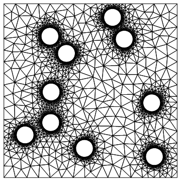
mesh = ToElementMesh[nr]

mesh["Wireframe"]

enter image description here

mesh["BoundaryElementMarkerUnion"]
{1, 2, 3, 4, 5, 6, 7, 8, 9, 10, 11, 12, 13, 14}

mesh["Wireframe"["MeshElement" -> "BoundaryElements", 
  "MeshElementMarkerStyle" -> Blue]]

enter image description here

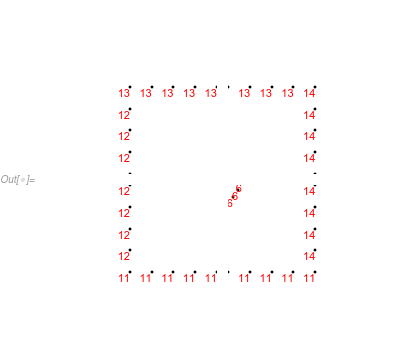
One thing to think about is that DirichletCondition uses the PointElement marker and not the BoundaryElement marker. So you need to make sure that this:

GraphicsGrid[
 Partition[
  mesh["Wireframe"["MeshElement" -> "PointElements", 
      "MeshElementMarkerStyle" -> Red, 
      PlotRange -> #]] & /@ {{{-1.2, -0.8}, {0.8, 1.2}}, {{0.8, 
      1.2}, {0.8, 1.2}}, {{-1.2, -0.8}, {-1.2, -0.8}}, {{0.8, 
      1.2}, {-1.2, -0.8}}}, 2]]

enter image description here

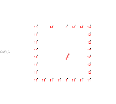
Is what you want. If not, you have the option to use something like x==1 and so forth in the respective DirichletCondition or generate a boundary mesh with the markers you want. Something like this:

bmOuter = 
  ToBoundaryMesh[
   "Coordinates" -> {{-1, -1}, {1, -1}, {1, 1}, {-1, 1}}, 
   "BoundaryElements" -> {LineElement[{{1, 2}, {2, 3}, {3, 4}, {4, 
        1}}, {1, 2, 3, 4}]}, 
   "PointElements" -> {PointElement[{{1}, {2}, {3}, {4}}, {11, 11, 13,
        13}]}];
bmesh = BoundaryElementMeshJoin @@ Flatten[{bmDisks, bmOuter}];
nr = ToNumericalRegion[r];
SetNumericalRegionElementMesh[nr, bmesh];
mesh = ToElementMesh[nr];
GraphicsGrid[
 Partition[
  mesh["Wireframe"["MeshElement" -> "PointElements", 
      "MeshElementMarkerStyle" -> Red, 
      PlotRange -> #]] & /@ {{{-1.2, -0.8}, {0.8, 1.2}}, {{0.8, 
      1.2}, {0.8, 1.2}}, {{-1.2, -0.8}, {-1.2, -0.8}}, {{0.8, 
      1.2}, {-1.2, -0.8}}}, 2]]

enter image description here

This would lead you to:

op = -Laplacian[u[x, y], {x, y}] + 0.1 u[x, y];
BCedges = {DirichletCondition[u[x, y] == 0, ElementMarker == 11], 
   DirichletCondition[u[x, y] == 1, ElementMarker == 13]};
BCcircles = 
  Table[DirichletCondition[u[x, y] == RandomReal[{0, 1}], 
    ElementMarker == k], {k, 1, Length@positionList}];
BC = Join[BCedges, BCcircles];
ufun = NDSolveValue[{op == 0, BC}, u, {x, y} \[Element] mesh]

{DensityPlot[ufun[x, y], {x, y} \[Element] mesh, 
  ColorFunction -> "Temperature", AspectRatio -> Automatic, 
  PlotPoints -> 100, PlotRange -> All, ImageSize -> 400], 
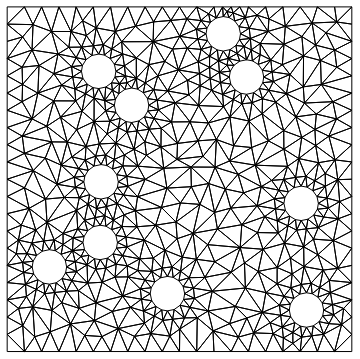
 Show[mesh["Wireframe"], ImageSize -> 400]}

enter image description here

$\endgroup$
4
$\begingroup$

There probably is a better way to do this, but I extracted the LineElements from bmesh and replaced the markers if they were in a particular disk region else a rectangular region.

Original OP Code

Needs["NDSolve`FEM`"]
radius = 0.1;
Louter = 2;
OuterRegion = Rectangle[{-L/2, -L/2}, {L/2, L/2}] /. L -> Louter;
positionList = {{0.706`, -0.14`}, {0.389`, 0.593`}, {-0.278`, 
    0.429`}, {0.254`, 
    0.844`}, {-0.46`, -0.367`}, {0.737`, -0.759`}, {-0.07`, -0.664`}, \
{-0.469`, 0.626`}, {-0.755`, -0.509`}, {-0.455`, -0.015`}};
diskRegions = Disk[#, radius] & /@ positionList;
mr = RegionDifference[OuterRegion, RegionUnion@diskRegions];
LP = ListPlot[positionList -> Table[k, {k, 1, Length@positionList}]];
RP = Show[mr // RegionPlot, LP, ImageSize -> 400]
bmesh = ToBoundaryMesh[RegionBoundary@mr, 
   "RegionHoles" -> positionList, "BoundaryGroupingThreshold" -> 0, 
   AccuracyGoal -> 1];
Show[bmesh["Wireframe"["MeshElementMarkerStyle" -> Blue]], 
 ImageSize -> 400]

Helper Functions

I created a list of region functions for the disks and a function diskIDfn to return the particular disk a point was in. Then I created a function to replace the markers depending the diskID or if it were on the rectangular boundary.

(* Determine if Point Lies in Dilated Disk Region *)
rmDiskFns = RegionMember[Disk[#, 1.05 radius]] & /@ positionList;
diskIDfn = (First@FirstPosition[Through[rmDiskFns[#]], True]) &;
(* Replace Marker From to be defined list *)
replaceMarker[l_] := 
 With[{rpl = ReplaceAll[{3 -> 11, 4 -> 12, 5 -> 13, 2 -> 14}]},
  If[NumericQ[First@l],
   LineElement[l[[2]], l[[3]] /. {First@l[[3]] -> First@l}],
   LineElement[l[[2]], rpl@l[[3]]]
   ]
  ]

Renumbering the Mesh

I extracted the coordinates and the list of LineElements from bmesh and created a substitution list to replace the markers.

(* Extract Coordinates and Boundary Elements *)
crd = bmesh["Coordinates"];
bes = bmesh["BoundaryElements"];
(* Create Substitution List *)
(* {newMarkerID,line element list, old marker list} *)
lelmMat = {diskIDfn@crd[[First@Flatten@#1]], #1, #2} & @@@ bes;
(* Replace Markers *)
bcEle = replaceMarker /@ lelmMat;
(* Re-boundary mesh and show new labels *)
bmeshnew = 
  ToBoundaryMesh["Coordinates" -> crd, "BoundaryElements" -> bcEle, 
   "RegionHoles" -> positionList];
Show[bmeshnew["Wireframe"["MeshElementMarkerStyle" -> Blue]], 
 ImageSize -> 400]

Renumbered Boundary Mesh

Note well that you will need to change the accuracy goal in the original bmesh definition to get a refined mesh. I changed the accuracy goal to 4 and repeated the process to generate the following element mesh.

mesh = ToElementMesh[bmeshnew];
mesh["Wireframe"]

Full Mesh

$\endgroup$

Your Answer

By clicking “Post Your Answer”, you agree to our terms of service and acknowledge you have read our privacy policy.

Not the answer you're looking for? Browse other questions tagged or ask your own question.