9
$\begingroup$

Let me abuse some Mathematica notation and formulate the following "command":

Show[RegionPlot4D[(Q1 - Q4)^2 < 16 Q3^2 && 
   Q1^2 + 4 Q1 Q2 + 16 Q2 (Q2 + Q3) + 12 Q2 Q4 + Q4^2 < 
    4 Q2 + 2 Q1 Q4 && Q1 > 0 && Q2 > 0 && Q3 > 0 && Q4 > 0, {Q1, 0, 
   6/61}, {Q2, 0, 2/9}, {Q3, 0, 1/32}, {Q4, 0, 1/6}], 
 RegionPlot4D[
  Q4 > 0 && Q2 > 0 && Q3 > 0 && Q1 + 4 (Q2 + Q3) + 3 Q4 < 1 && 
   4 Q2 + 9 Q4 < Q1, {Q1, 0, 6/61}, {Q2, 0, 2/9}, {Q3, 0, 1/32}, {Q4, 
   0, 1/6}], 
 RegionPlot4D[
  Q4 > 0 && Q2 > 0 && Q3 > 0 && Q1 + 4 (Q2 + Q3) + 3 Q4 < 1 && 
   2 (Q2 + Q3) + 3 Q4 < Q1, {Q1, 0, 6/61}, {Q2, 0, 2/9}, {Q3, 0, 
   1/32}, {Q4, 0, 1/6}]]

(Of course, there is a RegionPlot3D command, but no RegionPlot4D one.)

Can this be processed/interpreted in some manner? (use of coloring,...)

Also, these three "RegionPlot"s could be considered individually (challenging enough).

These pertain to certain quantum-information-theoretic problems concerned with probabilities of (bound) entanglement.

The problem as put is very much a direct 4D analogue of the 3D problem

Labeling distinct objects produced by Show[RegionPlot3D's]

that kglr answered. So, perhaps I should just try fixing (in various ways) one of the four coordinates and approaching the problem in the very same manner as there. (In fact, the constraints are set up in the same order both times, with the first one each times being the "PPT" one. Incidentally, the "PPT" body should be convex, but not the other two.)

In light of the rather widespread interest (mutiple answers) that has been shown in this problem, let me direct the readers, if so inclined, to pp. 16-17 in https://arxiv.org/abs/1905.09228. The elegant result (33) there pertains to the third RegionPlot3D command/constraint and the further result (34) to the second RegionPlot3D command/constraint. One can see the constraint (32) incorporated into the third command. The (PPT--positive-partial-transpose) constraint (30) is that employed in the first command, while the constraint (29) is incorporated into both the second and third ("entanglement") commands. (Needless to say, any substantive observations would certainly be welcome.)

$\endgroup$

4 Answers 4

9
$\begingroup$

You can define a 4D region with

R = ImplicitRegion[(Q1 - Q4)^2 < 16 Q3^2 && 
      Q1^2 + 4 Q1 Q2 + 16 Q2 (Q2 + Q3) + 12 Q2 Q4 + Q4^2 < 
      4 Q2 + 2 Q1 Q4 && Q1 > 0 && Q2 > 0 && Q3 > 0 && Q4 > 0,
      {Q1, Q2, Q3, Q4}]

and then check for region membership of any point. For example, make a list of lots of points in 4D and pick out those that lie inside of R:

P = Select[Tuples[Range[0, 1/4, 1/128], 4], Element[#, R] &];
Length[P]
(*    84579    *)

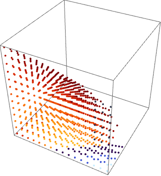
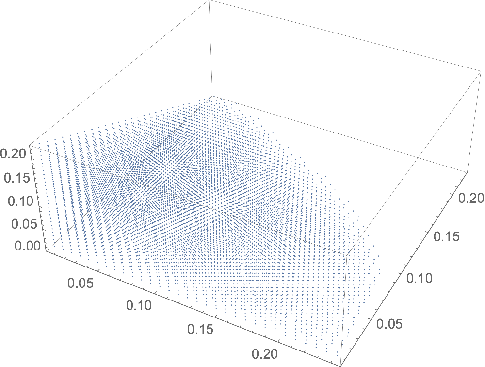
These can be plotted in many ways, for example by projecting out the fourth dimension and using only the first, second, third dimension as coordinate axes:

ListPointPlot3D[P[[All, {1, 2, 3}]]]

enter image description here

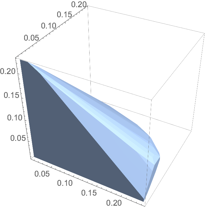
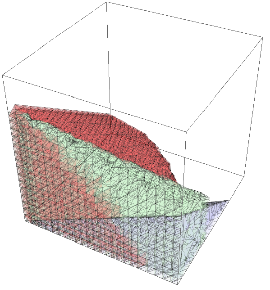
For a convex set, you can construct the convex hull in 3D for such a projection, for better visibility than the point cloud:

ConvexHullMesh[P[[All, {1, 2, 3}]], Boxed -> True, Axes -> True]

enter image description here

$\endgroup$
3
  • 1
    $\begingroup$ Could one use ListPointPlot3D with multiple point sets, using different colors? $\endgroup$ Commented Jul 16, 2019 at 21:28
  • 1
    $\begingroup$ @PaulB.Slater Yes you can. $\endgroup$
    – Roman
    Commented Jul 16, 2019 at 21:41
  • $\begingroup$ good method! and how to generate points in order to cover the area of ​​possible solutions of the function as uniformly and densely as possible. It seems to me that there should be quite a large number of test points per unit "volume" of this space. $\endgroup$
    – ayr
    Commented Jan 11, 2023 at 5:13
7
$\begingroup$

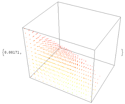
Using Graphics3D with VertexColors based on the fourth column is much faster than using ListPointPlot3D.

With a smaller version of Roman's P (to stay within my cloud credit limits):

P = Select[Tuples[Range[0, 1/4, 1/64], 4], Element[#, R] &];

Graphics3D[{PointSize[Small], Point[P[[All, ;; 3]], 
    VertexColors -> (Hue /@ P[[All, 4]])]}] // RepeatedTiming

enter image description here

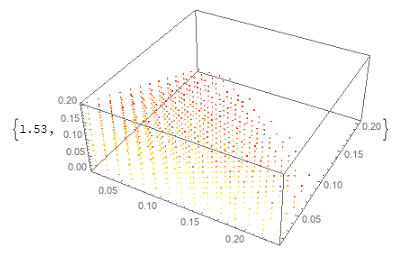
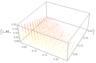
versus two alternative ways to use ListPointPlot3D:

ListPointPlot3D[Style[#[[;;3]], Hue @ #[[4]]]& /@ P,
   BaseStyle -> PointSize[Small]] // RepeatedTiming

enter image description here

ListPointPlot3D[List /@ P[[All, ;; 3]], 
  PlotStyle -> (Hue /@ P[[All, 4]]), 
  BaseStyle -> PointSize[Small]] // RepeatedTiming

enter image description here

Update: Plotting all three regions:

{ir1, ir2, ir3} = ImplicitRegion[{# && Q1 > 0 && Q2 > 0 && Q3 > 0 && Q4 > 0}, 
    {Q1, Q2,  Q3, Q4}] & /@
  {(Q1 - Q4)^2 < 16 Q3^2 &&  Q1^2 + 4 Q1 Q2 + 16 Q2 (Q2 + Q3) + 12 Q2 Q4 + 
     Q4^2 < 4 Q2 + 2 Q1 Q4,
   Q1 + 4 (Q2 + Q3) + 3 Q4 < 1 && 4 Q2 + 9 Q4 < Q1, 
   Q1 + 4 (Q2 + Q3) + 3 Q4 < 1 && 2 (Q2 + Q3) + 3 Q4 < Q1};

{p1, p2, p3} = Function[x, Select[Tuples[Range[0, 1/4, 1/64], 4], Element[#, x] &]] /@ 
   {ir1, ir2, ir3};

Graphics3D[{PointSize[Medium], 
  Point[p1[[All, ;; 3]], VertexColors -> (ColorData["SolarColors"] /@ 
      Rescale[p1[[All, 4]]])],
  Point[p2[[All, ;; 3]], VertexColors -> (ColorData["GrayYellowTones"] /@ 
      Rescale[p2[[All, 4]]])],
  Point[p3[[All, ;; 3]], VertexColors -> (ColorData["DeepSeaColors"] /@ 
      Rescale[p3[[All, 4]]])]}, BoxRatios -> 1]

enter image description here

Update 2: We can use TransformedRegion to get 3D regions from ir1, ir2 and ir3

{tir1, tir2, tir3} = TransformedRegion[#, {Indexed[#, 1] , Indexed[#, 2], 
       Indexed[#, 3] } &] & /@ {ir1, ir2, ir3};

then use ToElementMesh from NDSolve`FEM to discretize the transformed regions

Needs["NDSolve`FEM`"]
{m1, m2, m3} = ToElementMesh /@ {tir1, tir2, tir3};

wf1 = m1["Wireframe"["MeshElement" -> "MeshElements", 
    "MeshElementStyle" -> {Directive[EdgeForm[{Opacity[.3], Thin}], 
       FaceForm[{Opacity[.1], Red}]]}]];
wf2 = m2["Wireframe"["MeshElement" -> "MeshElements", 
    "MeshElementStyle" -> {Directive[EdgeForm[{Opacity[.3], Thin}], 
       FaceForm[{Opacity[.025], Green}]]}]];
wf3 = m3["Wireframe"["MeshElement" -> "MeshElements", 
    "MeshElementStyle" -> {Directive[EdgeForm[{Opacity[.3], Thin}], 
       FaceForm[{Opacity[.025], Blue}]]}]];

Show[wf1, wf2, wf3, PlotRange -> {{0, .3}, {0, .2}, {0, .3}}, 
 BoxRatios -> 1, Boxed -> True, ImageSize -> Large]

enter image description here

Ignored the fourth dimension altogether -- till we figure out how to associate each cell in 3D mesh with the fourth dimension.

$\endgroup$
4
  • $\begingroup$ So, can one jointly plot these results (presumably using different coloration schemes,...) with the parallel results based on one or both of the two other constraints given in the statement of the question? The expectation is that there should be some very small ("bound entanglement") overlap, if at all, between the points for the first constraint and those for either of the other two subsequent constraints. (Only the first constraint should yield a convex body, though.) $\endgroup$ Commented Jul 17, 2019 at 2:35
  • $\begingroup$ @Paul, please see the update. $\endgroup$
    – kglr
    Commented Jul 17, 2019 at 5:22
  • $\begingroup$ The p3 ("DeepSeaColors") points clearly stand out as being on the periphery of the p1 ("SolarColors") points--which jibes nicely with expectations. The p2 ("GrayYellowTones") points do not stand out quite as well, and seem peripheral also, but not quite as much. Maybe the p2's and p3's have little overlap (forming "islands")--which would also be of interest . So, if I nontrivially permuted the 4 variable names (say Q1->Q2, Q2->Q4, Q3->Q1, Q4->Q3) I would expect to get variations of the 3D plot displayed.----Thanks for your interest and skill. $\endgroup$ Commented Jul 17, 2019 at 12:31
  • $\begingroup$ So, since the p1 points should form a convex set, would use (as Roman indicated in his answer) of the ConvexHullMesh command lead to "better visibility than the point cloud"? (To reiterate, the other two point sets are not expected to form convex sets.) $\endgroup$ Commented Jul 17, 2019 at 18:39
3
$\begingroup$

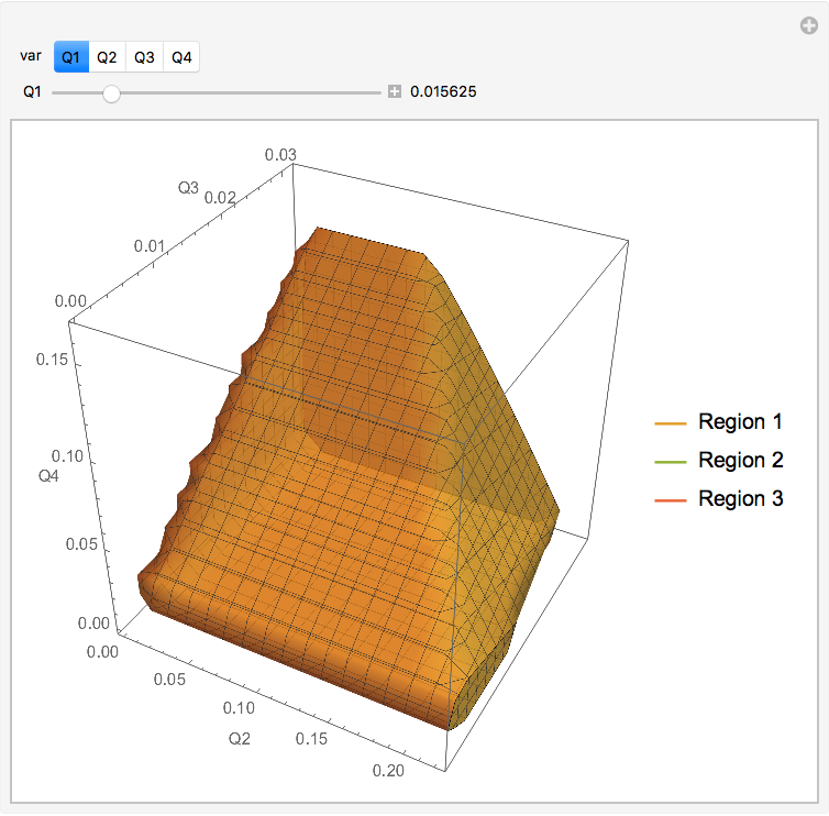
A traditional way to attempt to visualize 4D regions is via a series of sections (intersections with a 3D hyperplane). The easiest to construct are sections parallel to three of the coordinate axes.

Clear[Q1, Q2, Q3, Q4];
domain = {{Q1, 0, 6/61}, {Q2, 0, 2/9}, {Q3, 0, 1/32}, {Q4, 0, 1/6}};
max[var_] := First@Cases[domain, {var, _, m_} :> m];
Manipulate[
 var /. v_ :> Block[{Q1, Q2, Q3, Q4},
    v = x;
    Legended[
     Show[
        RegionPlot3D[(Q1 - Q4)^2 < 16 Q3^2 && 
          Q1^2 + 4 Q1 Q2 + 16 Q2 (Q2 + Q3) + 12 Q2 Q4 + Q4^2 < 
           4 Q2 + 2 Q1 Q4 && Q1 > 0 && Q2 > 0 && Q3 > 0 && 
          Q4 > 0, ##,
         PlotStyle -> Directive[ColorData[97][2], Opacity[0.7]], 
         AxesLabel -> Automatic],
        RegionPlot3D[
         Q4 > 0 && Q2 > 0 && Q3 > 0 && Q1 + 4 (Q2 + Q3) + 3 Q4 < 1 && 
          4 Q2 + 9 Q4 < Q1, ##,
         PlotStyle -> Directive[ColorData[97][3], Opacity[0.7]]], 
        RegionPlot3D[
         Q4 > 0 && Q2 > 0 && Q3 > 0 && Q1 + 4 (Q2 + Q3) + 3 Q4 < 1 && 
          2 (Q2 + Q3) + 3 Q4 < Q1, ##,
         PlotStyle -> Directive[ColorData[97][4], Opacity[0.7]]]
        ] & @@ DeleteCases[domain, {var, _, _}],
     LineLegend[
      Table[ColorData[97][k], {k, 2, 4}], 
      Table[Row[{"Region ", k}], {k, 1, 3}]]
     ]
    ],
 {var, domain[[All, 1]],
  TrackingFunction -> ((var = #; x = Clip[x, {0., N@max[var]}]) &)},
 {{x, 1./64, Dynamic@var}, 0., Dynamic@max[var], 
  Appearance -> "Labeled"}
 ]

enter image description here

Select the variable var whose axis is normal to the hyperplane. Then vary x to get sequence of sections var == x.

The second region is elusive. You need Q4 in the neighborhood of 0.005 and Q2 sampled around 0.006, which entails more PlotPoints than the default. (It can be done with PlotPoints -> {15, 40, 15} if Q4 is selected.)

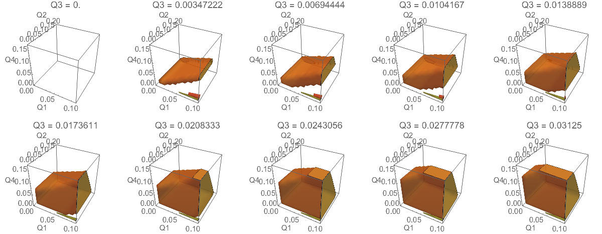
Here is a series for Q3. With some effect, one can imagine how the changes as Q3 increases.

enter image description here

$\endgroup$
5
  • $\begingroup$ Pretty amazing--with that dialing feature! $\endgroup$ Commented Jul 19, 2019 at 0:13
  • $\begingroup$ How does one incorporate PlotPoints -> {15, 40, 15} if Q4 is selected? $\endgroup$ Commented Jul 19, 2019 at 0:28
  • $\begingroup$ @PaulB.Slater I stuck the option in the second region plot in Manipulate, re-executed the code, selected Q4, set the slider for 0.005, a little green region appears. The `` PlotPoints -> {15, 40, 15} sets the number of initial points for each variable. So 40 for Q2 when Q4 is selected. If say Q1 is selected, then the variables are Q2, Q3, Q4 and the 40 will correspond to the second variable Q3. I didn't bother to figure out an automatic way, but this seems to work: PlotPoints -> Pick[{15, 40, 15, 50}, Replace[{Q1, Q2, Q3, Q4}, {var -> False, _ -> True}, 1]] $\endgroup$
    – Michael E2
    Commented Jul 19, 2019 at 0:49
  • $\begingroup$ Hmm, if I manipulate the controls too quickly, it seems to mess up. It sets the value of var to some random numeric value -- I think it's a problem of RegionPlot using Block to assign a value temporarily to Q1 etc. and the preemptive interrupting of clicking on a control. Not sure if that should be considered a bug, or something I should fix...I mean it's OK if Q1 is set to number, but it's not OK if var is set to a number. $\endgroup$
    – Michael E2
    Commented Jul 19, 2019 at 0:54
  • $\begingroup$ So, as Q3 increases the small isolated island seemingly merges with the large (PPT) body. The green of the island corresponds to the second constraint, and the red--which seems to fade away--to the third constraint (right?). In light of the rather widespread interest in this problem, let me direct the readers to pp. 16-17 in arxiv.org/abs/1905.09228. The result (33) pertains to the third RegionPlot3D command/constraint and the result (34) to the second RegionPlot3D command/constraint. (I'll add these last two sentences to the problem statement, as well.) $\endgroup$ Commented Jul 19, 2019 at 14:11
2
$\begingroup$

Well, here's my attempt to "wed" the ConvexHullMesh suggestion of Roman with the answer of kglr:

https://www.wolframcloud.com/obj/a291bc1f-1d05-4f89-881a-a39442dd6e77

The p3 "DeepSeaColors" points emerge strongly, but not so sure about the p2 "GrayYellowTones"--while I see three light blue (azure?) dots in the lower right-hand corner.

We expect the p2 and p3 points to be highly peripheral to the (convex) p1 points--with only a low (bound-entangled) probability of each's intersection with p1.

Well, in the full four-dimensional setting, the p1 points should occupy a volume (probability) of $\frac{1}{24} \left(12+\sqrt{3} \log \left(2-\sqrt{3}\right)\right) \approx 0.40495675$, the p2 points a volume of $\frac{1}{8}$ and the p3 points, $\frac{2}{9}$, with an intersection of p2 and p3 of $\frac{1}{9}$.

$\endgroup$

Your Answer

By clicking “Post Your Answer”, you agree to our terms of service and acknowledge you have read our privacy policy.

Not the answer you're looking for? Browse other questions tagged or ask your own question.