0
$\begingroup$

I am unfamiliar with Mathematica and the necessary syntax to approach visualize acceleration over time. I would appreciate some assistance or reference to a starting point on how to go about solving this problem. Please note that I have never used Mathematica before.

I am writing some game code that handles a third-person camera rotation that increases in speed over time (acceleration) as the left or right directional buttons are held down.

I am currently polling the directional button once every t milliseconds where sampling begins at the base and increases linearly every 100ms by a delta towards a maximum sampling rate.

So, for example (in microseconds):

TurnAccelMin = 10000.0
TurnAccelMax = 2000.0
TurnDelta = 1000.0

Note that acceleration is based on the sample rate so a lower maximum results in more samples over time. Even though sampling is in milliseconds, acceleration is stored as microseconds to account for a finer delta.

I would like to graph this so that I can visually see how the delta affects the acceleration over time. While I can picture in my mind the linear acceleration, I want to graph this so that I can visualize how different kinds of acceleration (exponential, quadratic, etc.) affect acceleration over a sample period.

How can I graph this as a line given these values as an equation?

Currently (as linear), where x = Time between 0 and 5 seconds and y = Acceleration in milliseconds.

Ideally I would like to see a graph of points, each connected by a straight line, as well as a table of values for each point when it is polled.

$\endgroup$
5
  • $\begingroup$ Welcome, Zhro...so shouldn't the acceleration be constant when the button is held down, and zero otherwise? So the rotation rate $\omega$ would be linearly increasing? Or would you see the acceleration itself increasing the longer you held the button down? $\endgroup$
    – MikeY
    Commented Jan 22, 2019 at 13:40
  • $\begingroup$ The acceleration is a function of the time between polling being reduced. The delta is constant (+1) but the frequency increases over time due to acceleration. Imagine adding 1 to a value every 10 seconds versus once a second. The delta is constant but the delta over time increases. There are two separate loops. The rate at which the delta is polled (variable) and the rate at which the acceleration is increased (static at every 1/10 of a second). Currently the delta changes by 1 every 7ms (min) to every 2ms (max). $\endgroup$
    – Zhro
    Commented Jan 22, 2019 at 14:07
  • $\begingroup$ Why don't you code in the acceleration step size to be $1/\delta t$ instead of just $1$, so your increase in $\omega$ per unit time is always constant? Just a little more or less smooth in its jumps? $\endgroup$
    – MikeY
    Commented Jan 22, 2019 at 14:48
  • $\begingroup$ I would be happy to experiment with alternative solutions but I would like to do this after I have a way to visualize this so that I'm no longer relying on just the "feel" of rotation in the game. I want a graph and table to back it up and cement in my mind how different approaches affect the result. $\endgroup$
    – Zhro
    Commented Jan 23, 2019 at 0:51
  • $\begingroup$ did I answer the question? $\endgroup$
    – MikeY
    Commented Jan 24, 2019 at 14:30

1 Answer 1

1
$\begingroup$

You wrote...

"where sampling begins at the base and increases linearly every 100ms by a delta towards a maximum sampling rate."

Are polling and sampling the same thing here? Do you mean...

where polling begins at the base and decreases linearly every 100ms by a delta towards a maximum polling rate."

In this case and with renamed variables to match what you are doing...

pollIntervalMax = 10000
pollIntervalMin = 2000
pollDelta = 1000

Assuming that is true, you can create a table of data. Breaking it up into its pieces...

numSteps = 12;
pollingPeriods = Table[Max[pollIntervalMax - pollDelta idx, pollIntervalMin], {idx, 1, numSteps}]; 

{9000, 8000, 7000, 6000, 5000, 4000, 3000, 2000, 2000, 2000, 2000, 2000}

Get polling times

pollingTimes = Accumulate[pollingPeriods]

{9000, 17000, 24000, 30000, 35000, 39000, 42000, 44000, 46000, 48000, 50000, 52000}

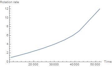
You can now plot the rotation rate as a function of time. Your rotation rate list is

rotRate = Range[numSteps]

{1, 2, 3, 4, 5, 6, 7, 8, 9, 10, 11, 12}

ListLinePlot[Transpose[{pollingTimes, rotRate}]]

enter image description here

$\endgroup$

Your Answer

By clicking “Post Your Answer”, you agree to our terms of service and acknowledge you have read our privacy policy.

Not the answer you're looking for? Browse other questions tagged or ask your own question.