Simple scenario is to see the Bézier function, but how to know which polynomial approximate it?
pts = {{0, -1}, {1, 0}, {2, -1}};
Graphics[{BezierCurve[pts], Green, Line[pts], Red, Point[pts]}]
Bézier Curves have a standard formula:
bezier[pts_List] := With[{n = Length[pts] - 1},
  Evaluate @ Sum[Binomial[n, i] (1 - #)^(n - i) #^i pts[[i + 1]], {i, 0, n}] &]
In Mathematica, the coefficient function of pts[[i + 1]] is the same as BernsteinBasis[n, i, #].
The above formula is of degree one less than the number of points in pts. In the Mathematica function, the degree used in BezierCurve is typically limited to be at most the setting of SplineDegree. By default, the setting is Automatic, and experimentation shows that it is the same as SplineDegree -> 3. In this case the list of points are partitioned into overlapping groups of 4 (or less).
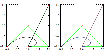
Example. I added some more points, to show what happens when there is not a multiple of 4.
pts = {{0, -1}, {1, 0}, {2, -1}, {1, -1}, {2, 1}};

g1 = Graphics[{Green, Line[pts], Black, BezierCurve[pts], Red,
    Point[pts]}, Frame -> True];
g2 = ParametricPlot[
      Evaluate[bezier[#][t] & /@ Partition[pts, 4, 3, 1, {}]],
      {t, 0, 1},
      AspectRatio -> Automatic, Frame -> True, Axes -> False,
      Prolog -> {Green, Line[pts], Red, Point[pts]}];

GraphicsRow[{g1, g2}]
bezier[#][t] & /@ Partition[pts, 4, 3, 1, {}]

(* {{3 (1 - t)^2 t + 6 (1 - t) t^2 + t^3,  -(1 - t)^3 - 3 (1 - t) t^2 - t^3},
    {1 + t,  -1 + 2 t}} *)
In this particular case since you supplied three points you get a quadratic bezier:
t^2 pts[[1]] + 2 t (1 - t) pts[[2]] + (1 - t)^2 pts[[3]]
You can see that this is correct at least to machine precision:
With[{t = RandomReal[{0, 1}]},
       t^2 pts[[3]] + 2  t (1 - t) pts[[2]] +  (1 - t)^2 pts[[1]] ==
              BezierFunction[pts][t]]
(* true *)
Assuming that BezierCurve is based on BezierFunction of course..
Of course the real question is how the divine this automatically, that I dont know..