5
$\begingroup$

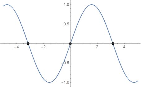
MeshFunctions helps to get an approximation of the roots

Plot[Sin[x], {x, -5, 5}, MeshFunctions -> {#2 &}, Mesh -> {{0}}, MeshStyle -> {PointSize[Large]}]

enter image description here

of the plotfunction, wish is accessed as a pure function #2&

How can I detect points of a given slope of (#2&) in the same way? Thanks!

$\endgroup$
4
  • $\begingroup$ Thank you, I have to go your proposed way. $\endgroup$ Commented Jul 7, 2018 at 10:05
  • $\begingroup$ I was clearly wrong though, so I deleted the comment. $\endgroup$
    – Szabolcs
    Commented Jul 7, 2018 at 10:35
  • $\begingroup$ @Szabolcs I don't think so. Your comment concerning the derivative of a pure function inside stills holds. $\endgroup$ Commented Jul 7, 2018 at 12:14
  • $\begingroup$ I mean, I forgot that the mesh can be specified not only in terms of the y coordinate but also the x coordinate. Then we can use an explicit form of the derivative function, as Brett did. $\endgroup$
    – Szabolcs
    Commented Jul 7, 2018 at 15:43

2 Answers 2

6
$\begingroup$

If you're only plotting one function at a time you could use the following:

f = Sin[x];

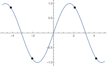
Plot[f, {x, -5, 5}, MeshFunctions -> {Function[x, Evaluate[D[f, x]]]},
  Mesh -> {{-0.5}}, MeshStyle -> {PointSize[Large]}]

enter image description here

The mesh function uses Evaluate since we need to make sure the derivative is taken with a symbolic value of $x$, before it starts receiving numeric values.

$\endgroup$
1
  • $\begingroup$ Thank you for your suggestion to use explicit functions. $\endgroup$ Commented Jul 7, 2018 at 10:06
4
$\begingroup$

Here is an approach that follows @Szabolcs' suggestion in comments, i.e of plotting the derivative of the function to extract the values, then reporting those values back to a plot of the original function:

Clear[f]
f[x_?NumericQ] := Sin[x]

pts = Cases[
  Normal@
   Plot[
     D[f[t], t] /. t -> x, {x, -5, 5},
     MeshFunctions -> {#2 &}, Mesh -> {{-0.5}}
   ], p_Point :> First[p], All];

tangents = Function[{x}, f[#1] + #2 (x - #1) & @@@ pts];

Plot[
  {f[x], Style[tangents[x], GrayLevel[0.5], Dashed]},
  {x, -5, 5}, PlotRange -> 1.2,
  Epilog -> {
    PointSize[Large], Red,
    Point[pts /. {x_Real, y_Real} :> {x, f[x]}]
  },
  ImageSize -> Large
]
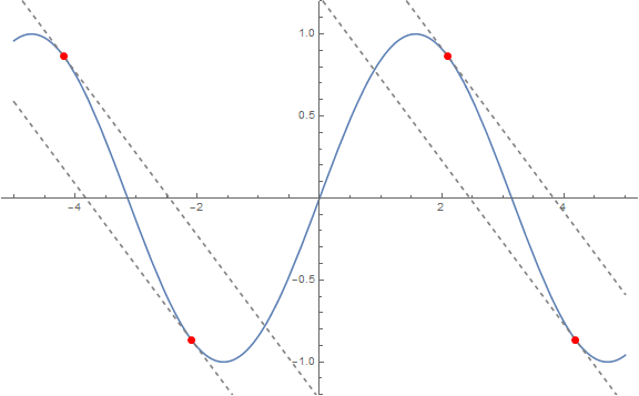
Mathematica graphics

I have defined the function in question as something that only evaluates when given numeric input to show that this should work with reasonable functions more complex than the simple Sin[x] as well.


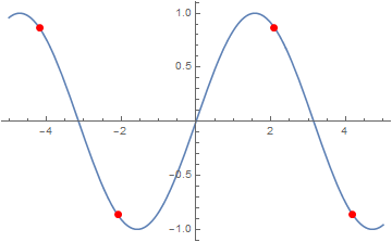
An alternative way to find those points is to use the NDSolve machinery and WhenEvent:

Reap[
  NDSolve[
    {D[y[x], x] == f'[x], y[0] == f[0], WhenEvent[y'[x] == -0.5, Sow[x]]}, 
    y, {x, -5, 5}
  ]
][[2, 1]]

(* Out: {-2.0944, -4.18879, 2.0944, 4.18879} *)


Plot[
  f[x], {x, -5, 5},
  Epilog -> {
   PointSize[Large], Red,
   Point[{#1, f[#1]} & /@ ptsNDSolve]
  }
]
Mathematica graphics

$\endgroup$
1
  • $\begingroup$ Thank you for your very helpful hints. $\endgroup$ Commented Jul 7, 2018 at 10:07

Your Answer

By clicking “Post Your Answer”, you agree to our terms of service and acknowledge you have read our privacy policy.

Not the answer you're looking for? Browse other questions tagged or ask your own question.