This question is related to "Numerical Fourier transform of a complicated function" from 2012.
I have pretty much the same problem: I have a function $f(x)$ which is complicated to evaluate, and want to calculate $$ F(t) = \frac{\mathrm e^t}{\pi} \int_0^\infty f(x)\, \mathrm e^{itx}\; \mathrm dx . $$ I have sampled $f(x)$, for example data see here. From these points I want to obtain $F(t)$. The problem is: I have tried to do this in 3 different ways, and each gives slightly different results. I want to know which method is most reliable, and how to best improve accuracy.
If you want to try this yourself, save the example data in a file "samples.txt" and load it:
samples = ToExpression /@
    Import[FileNameJoin[{NotebookDirectory[], "samples.txt"}], "Data"];
samplePlot = ListPlot[{
    Cases[samples, {x_, f_} -> {x, Re[f]}],
    Cases[samples, {x_, f_} -> {x, Im[f]}]},
  PlotTheme -> "Detailed", PlotLegends -> None, PlotRange -> {{0, 200}, Full},
  AspectRatio -> 1/5, ImageSize -> Full, PlotMarkers -> {Automatic, Tiny}]
Method 1: NFourierTransform
My first attempt was to simply use NFourierTransform. For this, I interpolated my sample data, continuing with zero outside of the sampled domain. (Note that I convert to an integral $\int_{-\infty}^\infty$ by setting $f(-x)=f(x)^\ast$.)
maxX = 3000;

realParts = Cases[samples, {x_, f_} -> {x, Re[f]}];
imagParts = Cases[samples, {x_, f_} -> {x, Im[f]}];
intRe = Interpolation[realParts];
intIm = Interpolation[imagParts];
interpolation[x_] :=
    Which[Abs[x] >= maxX, 0, x >= 0, intRe[x] + I*intIm[x], True, intRe[-x] - I*intIm[-x]];

Needs["FourierSeries`"];
method1 = Range[-3, 0.75, 0.1] // 10^# & //
  Table[{t, E^t / (2*\[Pi]) * Re@NFourierTransform[
    interpolation[x], x, t, FourierParameters -> {1, 1}]}, {t, #}] &;

plot1 = ListLogLogPlot[method1,
  PlotTheme -> "Detailed", PlotLegends -> None, ImageSize -> Large,
  PlotStyle -> Black, PlotMarkers -> {Automatic, Small}, PlotRange -> {10^-4, 20}]
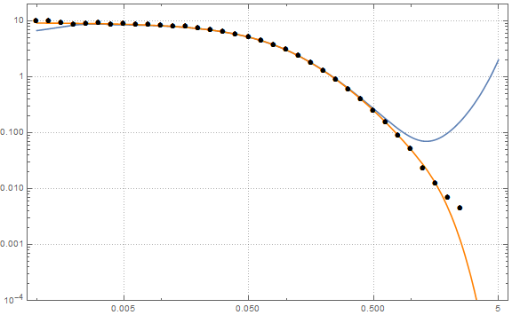
Note that this gives negative values $F(t)$ for the largest $t$-values, which should be impossible.
Method 2: DFT
Next I thought, I have discrete data points, I should maybe try a discrete Fourier transformation. Taking some code from this answer, I did the following:
dx = 0.1;
numpoints = maxX/dx;
upsampled = Range[0, maxX, dx] // Table[interpolation[x], {x, #}] &;

method2 = Re@Fourier[upsampled, FourierParameters -> {1, 1}]*dx //
    RotateRight[#, Floor[(numpoints - 1)/2]] & //
    Transpose@{Range @@ ({-Floor[(numpoints - 1)/2], Ceiling[(numpoints + 1)/2], 1}/(maxX)), #} & //
    Cases[#, {t_, v_} -> {2*\[Pi]*t, E^(2*\[Pi]*t)/\[Pi]*v}] & //
    Interpolation;

plot2 = LogLogPlot[method2[t], {t, 0.001, 5}, PlotRange -> {10^-4, 20},
  PlotTheme -> "Detailed", PlotLegends -> None, ImageSize -> Large]
Note that the original samples are not evenly spaced, I am using the interpolation from above to create more sample points.
Method 3: Fitting
I have found a simpler function which fits the sample data reasonably well:
samplesMirrored = Cases[samples, {t_, f_} -> {-t - 1, Re[f]}] \[Union]
    Cases[samples, {t_, f_} -> {t, Im[f]}];
fitfun[x_] := A1/(1 + B1 + I*x) + A2/(1 + B2 + I*x) + (A3*2!)/(1 + B3 + I*x)^3;
fitfunMirrored[x_] := Evaluate@If[x < -1/2,
  Evaluate@ComplexExpand@Re[fitfun[-x - 1]], Evaluate@ComplexExpand@Im[fitfun[x]]];
fit = FindFit[
  samplesMirrored,
  {fitfunMirrored[x], B1 > 0, B2 > 0, B3 > 0},
  {{A1, 6.6}, {B1, 15.3}, {A2, 2.7}, {B2, 5.2}, {A3, 1.2}, {B3, 3.5}},
  x];

Show[Plot[{Re@fitfun[x] /. fit, Im@fitfun[x] /. fit}, {x, 0, 20},
  PlotTheme -> "Detailed", PlotLegends -> None, ImageSize -> Large], samplePlot]
Show[Plot[{Re@fitfun[x] /. fit, Im@fitfun[x] /. fit}, {x, 1000, 3000},
  PlotTheme -> "Detailed", PlotLegends -> None, ImageSize -> Large], samplePlot]
The whole "mirrored"-business just deals with the fact that FindFit can't handle complex functions.
The fit function can be Fourier transformed analytically:
method3[t_] := A1*E^(-B1*t) + A2*E^(-B2*t) + A3*t^2*E^(-B3*t) /. fit;
plot3 = LogLogPlot[method3[t], {t, 0.001, 5}, PlotRange -> {10^-4, 20},
  PlotTheme -> "Detailed", PlotLegends -> None, ImageSize -> Large, PlotStyle -> Orange]
The results look as follows (black dots: NFourierTransform, blue: DFT, orange: Fit):

As you can see, the methods agree for intermediate values of $t$ and I would be certain enough that the result there is correct. However, I need $F(t)$ ideally for the whole range of $t$-values that is displayed here. What do you think: is one of these three methods more trustworthy than the others? If not, what would be the best way to increase the accuracy? (I did experiment a bit with taking more sample points, but it didn't immediately seem to help too much.)
