How can I improve the smoothness of my NDSolve solution?

Question

This will, unfortunately, be a broader question than I prefer, but I do have a concrete example.

I simulate many oscillatory systems with NDSolve. For short simulation times, the result is generally excellent. For longer times, the oscillations get jagged and visibly not-smooth. I find the array of options in NDSolve regarding accuracy, maximum step size, and maximum step count very confusing.

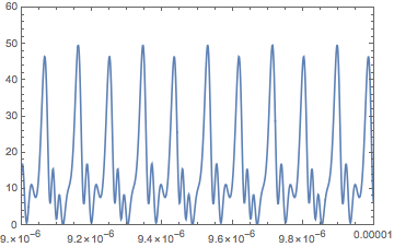
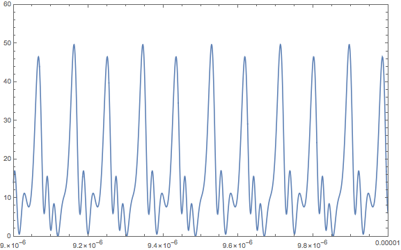
The NDSolve shown below is inferior to a 4th order Runge-Kutta (from Matlab). (For the interested, these equations describe the oscillation of an optomechanical oscillator driven by a laser.) The RK step size is 3.57e-10 (see the picture generated below the code). Yet when I set MaxStepSize in the NDSolve to 3e-10, still the NDSolve solution is jagged when viewed in the same window (and destroys features such as the alternating peak heights). Clearly the sampling rate is too low.

I have done my best to review the NDSolve options in the help; is there some other option that I have failed to tune correctly? (I also have a working Runge-Kutta in Mathematica, but as it employs loops, it is far too slow to use for longer simulations times.)

(1) How can improve the smoothness of this simulation, specifically? (2) Generally, which option does it seem I have overlooked and may save me this grief next time around? I can tolerate slow calculation, but not poor fidelity. Thanks very much.

m = 5*10^-11;
b = 1.4*10^-6;
k = 57559.5;

ringEqn = m r''[t] + b r'[t] + k r[t] == 1.02*10^-8 (Abs[A[t]])^2;

NW = 182.1;
DeltaW[t_] = 1.42*10^7 - 1.483*10^19 r[t];
ampEqn = A'[t] + A[t] (2.58*10^7 - I DeltaW[t]) == 3.74*10^8 I;

myInits = {r[0] == 0, r'[0] == 0, A[0] == 0};

myVars = {A, r};

OMOsol = NDSolve[{{ringEqn, ampEqn}, myInits}, 
  myVars, {t, 0, .000036}, MaxStepSize -> 3*10^-10, 
  MaxStepFraction -> .0000001]

amp = Evaluate[A[t] /. OMOsol];
Plot[(Abs[amp])^2, {t, 0, m/b},
   PlotRange -> {{.9*10^-5, 1*10^-5}, {0, 60}},
   Frame -> True]

Above: Mathematica--plot of (Abs[amp])^2 with above NDsolve

Above: Matlab--plot of (Abs[amp])^2 using 4th order Runge-Kutta with step size h=3.57e-10

Answer 1

Just increase PlotPoints in Plot. I tried 400 and got a nice result. BTW, it seems to run fine, and much faster, without MaxStepSize -> 3*10^-10, MaxStepFraction -> .0000001.

OMOsol = NDSolve[{{ringEqn, ampEqn}, myInits}, myVars, {t, 0, .000036}]

Plot[(Abs[amp])^2, {t, 0, m/b}, PlotRange -> {{.9*10^-5, 1*10^-5}, {0, 60}},
  Frame -> True, PlotPoints -> 400]

Answer 2

From Easy way to plot ODE solutions from NDSolve?, one might use ListLinePlot on the InterpolatingFunction:

ListLinePlot[
 {A["Grid"], Abs@A["ValuesOnGrid"]^2} /. First@OMOsol // Transpose // Interpolation,
 PlotRange -> {{.9*10^-5, 1*10^-5}, {0, 60}}, Frame -> True]

Since the plot range is a small portion, it may be worth selecting a subset of the solution:

range = {.9*10^-5, 1*10^-5};
grid = Flatten[A["Grid"] /. OMOsol];
mask = UnitStep[# - .9*10^-5] UnitStep[1*10^-5 - #] &@grid // SparseArray;
dom = Span @@ Flatten@Clip[
    mask["NonzeroPositions"][[{1, -1}]] + {-1, 1}, {1, Length@grid}]
(*  14461 ;; 16054  *)

ListLinePlot[
 ({A["Grid"], Abs@A["ValuesOnGrid"]^2} /. First@OMOsol)[[All, dom]] //
    Transpose // Interpolation,
 PlotRange -> {{.9*10^-5, 1*10^-5}, {0, 60}}, Frame -> True]

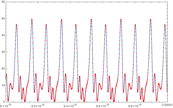
One can see the steps easily using Mesh, as in Matlab. Like @ChrisK, I omitted MaxStepSize -> 3*10^-10, MaxStepFraction -> .0000001. This is one way to see if the step size needs manual adjustment.

ListLinePlot[
 ({A["Grid"], Abs@A["ValuesOnGrid"]^2} /. First@OMOsol)[[All, dom]] // 
    Transpose // Interpolation,
 Mesh -> All, MeshStyle -> {PointSize[Small], Red}, 
 PlotRange -> {{.9*10^-5, 1*10^-5}, {0, 60}}, Frame -> True]