TimeLinePlot: change the y-axes ranges

Question

I want to combine a TimeLinePlot with a DateListPlot. My questions are:

1. Can you change the Y-axes of a TimeLinePlot?
2. Can you visualise the Y-axes of the DatelistPlot if you combine both plots using the Show function?

I use the next datasets:

data1e = {{DateObject[{2017, 01, 01}], 
     "event1"}, {DateObject[{2017, 01, 02}], 
     "event2"}, {DateObject[{2017, 01, 03}], 
     "event3"}, {DateObject[{2017, 01, 04}], 
     "event4"}, {DateObject[{2017, 01, 05}], 
     "event5"}, {DateObject[{2017, 01, 06}], 
     "event6"}, {DateObject[{2017, 01, 07}], "event7"}};
 data1d = {{DateObject[{2017, 01, 01}], 
    1}, {DateObject[{2017, 01, 02}], 2}, {DateObject[{2017, 01, 03}], 
    3}, {DateObject[{2017, 01, 04}], 4}, DateObject[{2017, 01, 05}], 
   5}, {DateObject[{2017, 01, 06}], 6}, {DateObject[{2017, 01, 07}], 
  7}}; data2e = {{DateObject[{2017, 01, 08}], 
   "event1"}, {DateObject[{2017, 01, 09}], 
   "event2"}, {DateObject[{2017, 01, 10}], 
   "event3"}, {DateObject[{2017, 01, 10}], 
   "event4"}, {DateObject[{2017, 01, 10}], 
   "event5"}, {DateObject[{2017, 01, 10}], 
   "event6"}, {DateObject[{2017, 01, 10}], 
   "event7"}, {DateObject[{2017, 01, 11}], 
   "event8"}, {DateObject[{2017, 01, 12}], 
   "event9"}, {DateObject[{2017, 01, 13}], 
   "event10"}, {DateObject[{2017, 01, 14}], "event11"}};
data2d = {{DateObject[{2017, 01, 08}], 
    110}, {DateObject[{2017, 01, 09}], 
    120}, {DateObject[{2017, 01, 10}], 
    130}, {DateObject[{2017, 01, 11}], 
    140}, {DateObject[{2017, 01, 12}], 
    150}, {DateObject[{2017, 01, 13}], 
    160}, {DateObject[{2017, 01, 14}], 170}};

I write 4 scripts to generate the different graphs.

TLP1 = TimelinePlot[
  MapThread[Labeled, {data1e[[All, 1]], data1e[[All, 2]]}]
  , PlotTheme -> "Detailed"
  , ImageSize -> 500
  , PlotRange -> {{DateObject[{2017, 01, 01}], 
     DateObject[{2017, 01, 14}]}, Automatic}];

DLP1 = DateListPlot[data1d
  , PlotTheme -> "Detailed"
  , ImageSize -> 500
  , PlotRange -> {{DateObject[{2017, 01, 01}], 
     DateObject[{2017, 01, 14}]}, {0, 200}}];

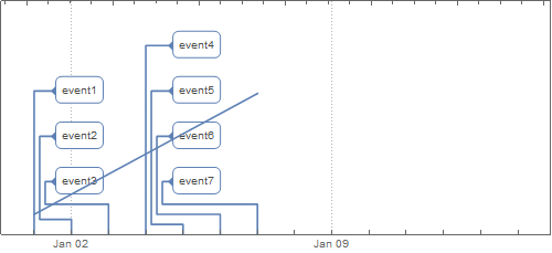
Show[{TLP1, DLP1}]

TLP2 = TimelinePlot[
  MapThread[Labeled, {data2e[[All, 1]], data2e[[All, 2]]}]
  , PlotTheme -> "Detailed"
  , ImageSize -> 500
  , PlotRange -> {{DateObject[{2017, 01, 01}], 
     DateObject[{2017, 01, 14}]}, {0, 200}}];

DLP2 = DateListPlot[data2d,
  , PlotTheme -> "Detailed"
  , ImageSize -> 500
  , PlotRange -> {{DateObject[{2017, 01, 01}], 
     DateObject[{2017, 01, 14}]}, {0, 200}}];

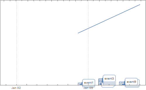
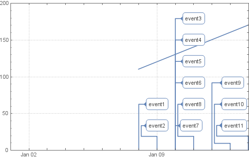
Show[{TLP2, DLP2}]

Both graphics has different sizes. Becasue I want to combine them in a (powerpoint) presentation I would like to have them the same sizes. And I want to show the the X-axes and the Y-axes.

Anyone a suggestion how to solve this issue?

Answer 1

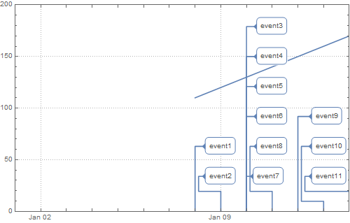
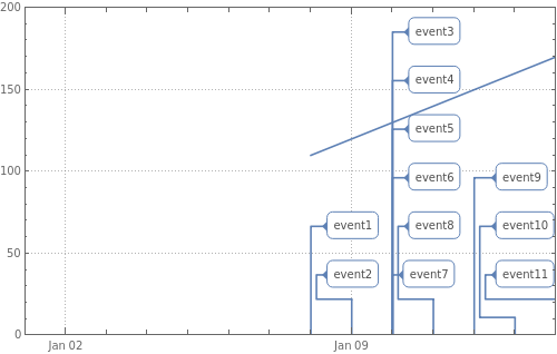
Update: For versions 11.3 and 12.2 we can use the following two functions to post-process the TimeLinePlot output to modify the vertical scale:

$Version

"11.3.0 for Microsoft Windows (64-bit) (March 7, 2018)"

ClearAll[modifyScaleV11]
modifyScaleV11[g1_, g2_] := MapAt[GeometricTransformation[#, 
    RescalingTransform @@ (PlotRange /@ {g1, g2})] &, g1, {1}]

Show[DLP2, modifyScaleV11[TLP2, DLP2]]

$Version (* Wolfram Cloud *)

"12.2.0 for Linux x86 (64-bit) (November 16, 2020)" 

ClearAll[modifyScaleV12]
 
modifyScaleV12[g1_, g2_] := Module[{pr = {PlotRange[g1][[1]], 
    {0, 1 + Max@Cases[g1, Inset[_, Offset[_, {_, a_}], ___] :> a,  All]}}},
  MapAt[GeometricTransformation[#, RescalingTransform[pr, PlotRange[g2]]] &, g1, {1}]]

Show[DLP2, modifyScaleV12[TLP2, DLP2]] 

Original answer:

You can modify the output of TimeLinePlot by rescaling the y-coordinates of the graphics primitives in it.

The function scaleF[g1, g2] below creates a scaling function that rescales any number in the vertical PlotRange of g1 to the vertical PlotRange of g2. The function modifyF[g1, g2] replaces the graphics primitives in g1 with their rescaled versions.

ClearAll[scaleF, modifyF]
scaleF[g1_, g2_] := Rescale[#, ## & @@ (PlotRange[#][[2]] & /@ {g1, g2})] &;

modifyF[g1_, g2_] := g1 /. {(head : Alternatives[Polygon, Point, Line])[x__] :> 
 head[x /. {Offset[y_, {a_, b_}] :> Offset[y, {a, scaleF[g1, g2]@b}], 
  {c_, d_} :> {c, scaleF[g1, g2]@d}} ], 
Inset[ins_, pos_, rest___] :> Inset[ins, pos /. Offset[y_, {a_, b_}] :> 
  Offset[y, {a, scaleF[g1, g2]@b}], rest ]};

Example:

Show[DLP2, modifyF[TLP2, DLP2]]