4
$\begingroup$

Most recipes on statistical data processing in Mathematica, such as building histograms, deriving smoothed PDF and CDF distributions, etc., work with given raw data sets. For example, series of measurements. However, there can be situations, when input is an already processed histogram with given counts for given bins.

Would it be a good idea to reconstruct a fake raw distribution according to some simplified algorithms? For example, a list of all data falling into a bin located at its centre or all data uniformly distributed across the bin interval.

I would like to have such lists in order to do further processing and to have at hand the whole distribution analysis toolkit. Is there some function to achieve this straightforwardly? Or can such cumulated data can be handled with available statistical methods for raw data? Can something be done with WeightedData?

Update. Here is some example data supplied to us with no trace of origin.

bins: 60-100;100-200;200-300;300-500;500-1000;1000-2000;2000-3000; >3000
counts: 275; 320; 112; 65; 53; 44; 16; 15

Interesting particulars are: 1) this is a censored data (rightmost interval is open; and 2) there is a suspicion on the heavy-tailed distribution. Moments of such a distribution function would diverge, and its asymptotics would be x^-n. For both cases statisticians have special caveats in handling. Are such caveats, specially for 1), treatable by Mathematica as well?

$\endgroup$
7
  • 3
    $\begingroup$ Have you seen HistogramDistribution[] and SmoothKernelDistribution[]? $\endgroup$ Commented Aug 18, 2017 at 16:35
  • 1
    $\begingroup$ Do you have a specific distribution in mind? Or is this just for any general histogram without a specific distribution in mind? I ask because if one has the histogram (counts and bin structure) and that the distribution is, say, a normal distribution, then there is an approach to obtain maximum likelihood estimates of the two parameters (mean and standard deviation in this case) that is very different than pretending a uniform distribution within a bin. $\endgroup$
    – JimB
    Commented Aug 18, 2017 at 17:34
  • $\begingroup$ we do not have any pre-set distribution. Just counted hist. data, from which I infer some distribution. A particular problem is comparing data with, e.g., normal dist (null hypothesis that data come from it). But the first step is to build density distribution (bins are unequal, but distributed close to logarithm, like: 200-300-500-1000-2000-3000- >3000). So it is to build true density hist. adjusting bar heights, and then via kernel smoothing infer a nonparametric estimation of the distribution. HistogramDistribution seems to do this for raw data, the same is for SmoothKernelDistribution $\endgroup$
    – astrsk
    Commented Aug 18, 2017 at 19:45
  • 1
    $\begingroup$ Alternatively, you can apply HistogramDistribution to a WeightedData object to do this in a fully documented way. $\endgroup$
    – Szabolcs
    Commented Aug 22, 2017 at 10:20
  • 1
    $\begingroup$ Given the example you've added, you should consider taking the logs of the bin boundaries and see mathematica.stackexchange.com/questions/35588/… for a visual display. $\endgroup$
    – JimB
    Commented Aug 23, 2017 at 3:31

3 Answers 3

6
$\begingroup$

You may use Piecewise to construct the "PDF" from your bins and counts. Then ProbabilityDistribution and RandomVariate to generate values.

First create some bin and count example data.

SeedRandom[411]
{b, c} = HistogramList[RandomVariate[BetaDistribution[2, 4], 300]];

Then construct the probability density function from this information.

ClearAll[piecewiseUniformDistribution];
piecewiseUniformDistribution[bins_, counts_] :=
 Module[{pdf},
  pdf = {#[[2]] 1/(#[[1, 2]] - #[[1, 1]]), #[[1, 1]] < \[FormalX] <= #[[1, 2]] } & /@ 
    Transpose@{Partition[bins, 2, 1], Standardize[counts, 0 &, Total]};
  pdf[[1, 2, 2]] = LessEqual;
  ProbabilityDistribution[{"PDF", Piecewise@pdf}, {\[FormalX], Sequence @@ MinMax@bins}]
  ]

There is only one trick in piecewiseUniformDistribution. To get the correct lower bound the first expressions condition is modified.

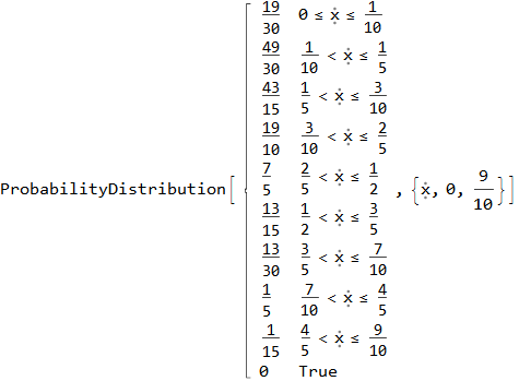
dist = piecewiseUniformDistribution[bins, counts]

Mathematica graphics

piecewiseUniformDistribution returns a ProbabilityDistribution object. This can be used just like the built-in Mathematica distributions. That is, it works with Mean, Variance, CDF, and so on.

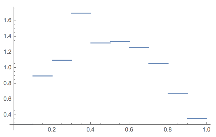
Plot[#[dist, x], {x, 0, 9/10}, ExclusionsStyle -> Directive[{Gray, Dashed}]]& /@ {CDF, PDF}

Mathematica graphics

Since the source distribution is known a goodness of fit KolmogorovSmirnovTest can be performed against some values generated with RandomVariate.

genData = RandomVariate[dist, 100];
KolmogorovSmirnovTest[genData, BetaDistribution[2, 4], {"PValue", "ShortTestConclusion"}]
{0.296624, "Do not reject"}

I am surprised that passing the results from HistogramList into HistogramDistribution is not supported as of version 11.1.1. You should contact WRI and request this be included.

Hope this helps.

$\endgroup$
1
  • $\begingroup$ Here's another possible implementation: piecewiseUniformDistribution[bins_, counts_] := ProbabilityDistribution[Internal`ToPiecewise[Append[MapAt[(# /. Less -> LessEqual) &, (#1 < \[FormalX] <= #2) & @@@ Partition[bins, 2, 1], 1], True], Append[Standardize[counts, 0 &, Total]/Differences[bins], 0]], {\[FormalX], ##} & @@ MinMax[bins], Method -> "Normalize"] $\endgroup$ Commented Aug 22, 2017 at 11:42
4
$\begingroup$

When you have already binned data, you can usually use WeightedData. Here's an example:

Let's create some example binned data:

data = RandomVariate[BetaDistribution[2, 2], 500];
binsize = 0.1;
{bins, counts} = HistogramList[data, {binsize}];
values = N@MovingAverage[bins, 2];

Build WeightedData object:

wd = WeightedData[values, counts]

There are many operations that can be performed on this (both statistical and other):

Mean[wd]
(* 0.4884 *)

Max[wd]
(* 0.95 *)

Median[wd]
(* 0.45 *)

If you need a distribution object, you can use HistogramDistribution with a manually specified bin size:

distr = HistogramDistribution[wd, {binsize}]

Plot[PDF[distr, x], {x, 0, 1}]

enter image description here


There is an old QA on a similar topic that shows how to directly construct a DataDistribution object from already binned data:

I do not remember if at the time WeightedData was available. Today I would definitely use WeightedData instead of undocumented functionality unless you have a good reason to construct the DataDistribution object directly.

$\endgroup$
4
$\begingroup$

The above two answers are what you want to do if all one has is the binned data. But sometimes one also knows (or at least would like to believe) the underlying distributional form.

In that case the maximum likelihood estimators for the parameters can be obtained from this "censored" data (with censored meaning that some or all of the data is only known to be in some interval). Using those parameter estimates one can then produce random samples from that estimated distribution.

If the bin borders are labeled $x_1, x_2, \ldots, x_{n+1}$, the frequency count between borders $i$ and $i+1$ is $f_i$, and $F(.)$ is the cumulative distribution function, then the likelihood is

$$\text{Likelihood}=\prod_{i=1}^n \left(F(x_{i+1})-F(x_i)\right)^{f_i}$$

and the log of the likelihood is

$$\log(\text{Likelihood})=\sum_{i=1}^n f_i \log\left(F(x_{i+1})-F(x_i)\right)$$

So we choose the parameter values that maximize the log of the likelihood. Using @Edmund 's example with a beta distribution:

(* Generate data *)
SeedRandom[411]
x = RandomVariate[BetaDistribution[2, 4], 300];
{b, c} = HistogramList[x]
(* {{0,1/10,1/5,3/10,2/5,1/2,3/5,7/10,4/5,9/10},{19,49,86,57,42,26,13,6,2}} *)

(* Construct log of the likelihood *)
logL = Sum[c[[i]] Log[CDF[BetaDistribution[α, β], b[[i + 1]]] - 
      CDF[BetaDistribution[α, β], b[[i]]]], {i, 1, Length[c]}];

(* Find maximum likelihood estimates *)
sol = NMaximize[{logL, α > 0 && β > 0}, {α, β}]
(* {-567.5592631676245, {α -> 2.334903877668157, β -> 4.813453250016402}} *)

(* Estimate parameter covariance matrix *)
cov = -Inverse[(D[logL, {{α, β}, 2}]) /. sol[[2]]];
cov // MatrixForm

$$\begin{pmatrix} 0.0382947 & 0.0711748 \\ 0.0711748 & 0.174881 \\ \end{pmatrix}$$

(* Approximate 95% confidence limits *)
αCL = (α /. sol[[2]]) + 1.96 {-1, 1} cov[[1, 1]]^0.5
(* {1.9513506715911781, 2.7184570837451356} *)
βCL = (β /. sol[[2]]) + 1.96 {-1, 1} cov[[2, 2]]^0.5
(* {3.9938060055815297,5.633100494451275} *)

(* Show original histogram and fit *)
Show[Histogram[x, Automatic, "PDF", PlotRange -> {{0, 1}, Automatic}],
 Plot[PDF[BetaDistribution[α, β], x] /. sol[[2]], {x, 0, 1}]]

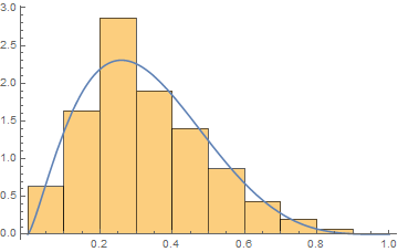
Histogram and fit

Note that one can obtain measures of precision for the parameters (of course, which only make sense if the underlying distribution is at least very close to the proposed distribution). Also, note that not using a parametric distribution and re-sampling from the original histogram does not mean one doesn't have to worry about sampling error.

Finally, random samples can now be obtained:

RandomVariate[BetaDistribution[α, β] /. sol[[2]], 100]
$\endgroup$
3
  • 1
    $\begingroup$ For computing the log-likelihood of the beta distribution, it is more convenient and more numerically stable to use a dot product along with the generalized form of BetaRegularized[]: logL = c.Log[Table[BetaRegularized[b[[i]], b[[i + 1]], α, β], {i, Length[c]}]] $\endgroup$ Commented Aug 22, 2017 at 17:53
  • $\begingroup$ Thanks @J.M. (again!) That's good to know. However, there is a problem with my code (D[logL, {{\[Alpha], \[Beta]}, 2}]) /. sol[[2]] when I use that modification. I get some errors: Infinity::indet: "Indeterminate expression 0.\ \[Infinity] encountered." and then no covariance estimate. I assume that's because of logL including BetaRegularized[0, 1/10, \[Alpha], \[Beta]]] which has a 0. (And maybe the same issue if there was a "1" as in BetaRegularized[9/10, 1, \[Alpha], \[Beta]]].) $\endgroup$
    – JimB
    Commented Aug 22, 2017 at 18:18
  • $\begingroup$ Interesting, tho the expression is good for maximization purposes, it seems to not do well when one tries to get its Hessian. I will look into this... $\endgroup$ Commented Aug 23, 2017 at 1:16

Your Answer

By clicking “Post Your Answer”, you agree to our terms of service and acknowledge you have read our privacy policy.

Not the answer you're looking for? Browse other questions tagged or ask your own question.