5
$\begingroup$

I had to run NSolve to solve a nonpolinomial equation (it has some square roots in it) to get roots of the equation. I've got a solution that looks something like this (see myrootsSolution). enter image description here
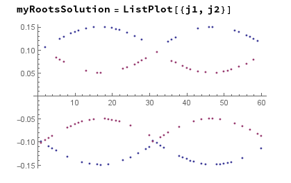
The equation is too big to be posted here, so I run code that simulates the roots solution. When you look at the plot of myrootsSolution, it is obvious that the roots have sinusoidal properties. Other thing is that points oscillate between two sines so that I cannot use the ListLinePlot or do other calculations. I think I can fix that problem by chopping the data in half and swapping the same way I created this data. Unless someone knows a better way. But how about the oscillating points? The code below simulates my roots solution:

Remove["Global`*"];
ClearAll;
max=6;steps=0.1
x=Range[0,max,steps];

y=0.05*Sin[x]+0.1;
ListPlot[y,PlotRange->{-0.2,0.2}]
w=-0.05*Sin[x]+0.1;
ListPlot[w,PlotRange->{-0.2,0.2}]
z = RandomInteger[1, max/steps + 1];
y1 = (-1)^z*y;
ListPlot[y1]
w1 = (-1)^z*w;
otherCase = ListPlot[w1]
n1 = List[y1, w1];
shouldBe = ListPlot[n1] (* but still noisy*)
p1=Take[y1,(max)/(2*steps)];
p2=Take[y1,-(max)/(2*steps)];
p3=Take[w1,(max)/(2*steps)];
p4=Take[w1,-(max)/(2*steps)];
j1=Join[p1,p4];j2=Join[p2,p3];
j3=List[j1,j2];
myRootsSolution=ListPlot[{j1,j2}]  (* this is what I get from NSolve *)
f1 = 0.05*Sin[x] + 0.1;
f2 = 0.05*Sin[x] - 0.1;
f3 = -0.05*Sin[x] + 0.1;
f4 = -0.05*Sin[x] - 0.1;
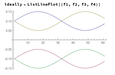
ideally = ListLinePlot[{f1, f2, f3, f4}]

In other cases, the roots solution is simple but still noisy; see othercase: enter image description here
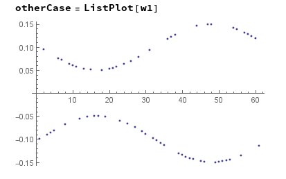
My goal is to sort the data points to get something ideal as shown here:

enter image description here

I don't think we can tell NSolve how to sort roots unless I am missing something. Do you know how to sort myRootsSolution data automatically (so that I can continue calculations with it) instead doing manual work like I can do by doing the reverse of creating those data. (note that NSolve finds all the roots).

Again, Below is my update to this question. I have made an attempt to automate this. I folded in half along the x-axis because both are symmetrical in y-axis always. So I ended up with two sine waves in the positive y-axis. My trick is to take the derivative of roots. If sine waves are separated the derivative should be a smooth cosine. If sine waves are crossing each other then the derivative is jerking at the crossing point. Since I don't have FindPeaks because Mathwolf v9, I have to find one. I am using those crossing points to determine from where should I flip the other half of the curves. See my code below of my attempt:

  ClearAll;
  max=6;steps=0.05;
  x=Range[0,max,steps];
  z=RandomInteger[1,Length[x]];
  f1=0.05*Sin[x]+0.1;
  f2=0.05*Sin[x]-0.1;
  f3=-0.05*Sin[x]+0.1;
  f4=-0.05*Sin[x]-0.1;
  ideally=ListLinePlot[{f1,f2,f3,f4}]
  ph=0.1;offs=0.1;
  e1=(Abs[0.05*Sin[x+ph]]+offs)*(-1)^z;
  e2=(Abs[0.05*Sin[x+ph]]-offs)*(-1)^z;
  e3=(-Abs[0.05*Sin[x+ph]]+offs)*(-1)^(z);
  e4=(-Abs[0.05*Sin[x+ph]]-offs)*(-1)^(z);
  e5={e1,e2,e3,e4};
  roots=Transpose[{e1,e2,e3,e4}];
  ListPlot[e5,PlotRange->{-0.2,0.2}]
  roots1=Abs[roots];
  ListPlot[Transpose@roots1,PlotRange->{-0.2,0.2}]
  size=Dimensions[roots1];
  columns=Part[size,2];
  column=Range[columns/2+1,columns,1];
  roots2=Part[roots1,All,{1,2}];
  ListPlot[Transpose@roots2,PlotRange->{-0.2,0.2}]
  dy3=With[{pad=IntegerPart[max/steps]-   1},ArrayPad[DerivativeFilter[ArrayPad[roots2,pad,"Extrapolated"],{1}],-pad]];
  test3=dy3;
  minD=(-MinDetect@test3);
  maxD= (MaxDetect@test3);
  fig1=ListLinePlot[Transpose@dy3,DataRange->{0,6}]
  fig2=ListPlot[0.003*Transpose@maxD,DataRange-> {0,6},PlotStyle->PointSize[0.02],PlotRange->{-0.004,0.004}]
 fig3=ListPlot[0.003*Transpose@minD,DataRange->  {0,6},PlotStyle->PointSize[0.02],PlotRange->{-0.004,0.004}]
  y=0.05*Sin[x]+0.1;
  w=-0.05*Sin[x]+0.1;
  ftest=List[y,w];
  minD1=0.15*(-MinDetect@ftest)+0.2;
  maxD1= 0.15*(MaxDetect@ftest);
  fig4=ListLinePlot[ftest,DataRange->{0,6}]
  fig5=ListPlot[maxD1,DataRange->  {0,6},PlotStyle->PointSize[0.02],PlotRange->{-.17,.17}]
  fig6=ListPlot[minD1,DataRange->  {0,6},PlotStyle->PointSize[0.02],PlotRange->{-.17,.17}]
  Show[fig1,fig2,fig3]
  Show[fig4,fig5,fig6]
  minx=x*Abs[minD];
  maxx=x*Abs[maxD];
  coord=List[{minx},{maxx}];
  Transpose@coord;

By looking at the derivatives, I know the top one changes from minimum to maximum in one step, and the bottom one changes from maximum to minimum both at crossing points. The problem I have is that the crossing point is not exactly and I have to narrow it down and then use those points to select halfs of sine to flip mirror so that I get original sine waves as shown in ideal variable. enter image description here
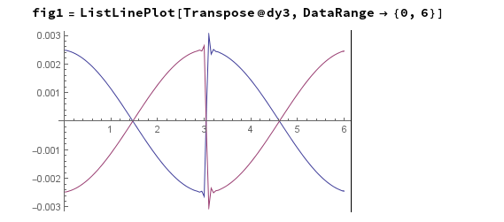
I also add code that shows why NSolver makes this kind of graph. I called the equation blackbox because actual equation is too complex and long for posting. But end result is very similar. Is there a way to modify NSolve code to fix this? Something like derivative roots?

Remove["Global`*"];//Quiet
ClearAll;
blackbox[a_]=(x-Sin[a]-1)*(x-Sin[a-Pi]-1)
(-1+x-Sin[a]) (-1+x+Sin[a])
xx=Range[0,2*Pi,0.01];
roots=Table[x/.NSolve[blackbox[b]==0,x],{b,xx}];
ListPlot[Transpose@roots]

Thanks in advance,

$\endgroup$
4
  • 3
    $\begingroup$ One approach would be to group together points from neighboring x values that give close numeric derivatives to prior such values. Perhaps better would be to start with one solution set and change the problem to one of solving a system of ODEs, in effect tracking the solution sets. $\endgroup$ Commented Jun 28, 2017 at 15:33
  • $\begingroup$ It is not clear what do you mean. I added extra code of my attempt to solve the problem....I am very close....but still stuck...I do not have FindPeaks because I have Mathwolf v9 $\endgroup$
    – Aschoolar
    Commented Jun 28, 2017 at 22:20
  • 1
    $\begingroup$ @DanielLichtblau I think I did what you were suggesting. Worked out well. $\endgroup$
    – MikeY
    Commented Jun 30, 2017 at 17:39
  • $\begingroup$ @MikeY Yes you did (and I upvoted as soon as I saw it). $\endgroup$ Commented Jun 30, 2017 at 19:14

2 Answers 2

11
$\begingroup$

OK, I've had this problem before myself. Here's a solution to a harder problem? Take your code to generate the roots list.

Remove["Global`*"];//Quiet
ClearAll;
blackbox[a_]=(x-Sin[a]-1)*(x-Sin[a-Pi]-1)
(-1+x-Sin[a]) (-1+x+Sin[a])
xx=Range[0,2*Pi,0.01];
roots=Table[x/.NSolve[blackbox[b]==0,x],{b,xx}];

Add a complication by just scrambling the results.

rootScramble = Map[#[[RandomSample[Range[2]]]] &, roots];

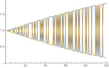
Plot a subset. Ugly!

enter image description here

Now, making the assumption that the results are smooth in the zeroth and 1st derivative, look at each point pair, and then permute the next pair in line to minimize a Norm involving both their values and derivatives. The idea is that while in the "point" space they might have the same value, in the phase space of both point and derivative, they differ and can be discriminated.

First create the permutator, which takes in as the first argument (assuming two curves, but should work for any number) {{p1,p2},{del1,del2}}. The dels are finite differences between the that point and the last one, stored up as the algorithm runs. The second argument is the point that needs permuting, {q1,q2}.

permMatch[{vals_, dels_}, l2_] := 
 Module[{l1 = {vals, dels}, ps, bestPerm},

  ps = Map[({#, # - vals}) &, Permutations[l2]];

  bestPerm = Sort[ps, Norm[l1 - #1] < Norm[l1 - #2] &] // First
  ]

The output of permMatch is a permutation {{qx,qy},{qx-p1,qy-p2}} that is "closest" to {{p1,p2},{del1,del2}}.

Now just use FoldList to process rootScramble, initializing with the {{0,0},{0,0}} to get it started then dropping it at the end.

res = FoldList[permMatch, {{0, 0}, {0, 0}}, rootScramble]//Rest;

Discard the differences and transpose

finalResult = Map[(# // First) &, res] // Transpose;

Plot the full before and after.

rootScramble // Transpose // ListLinePlot

enter image description here

finalResult // ListLinePlot

enter image description here

This could easily be extended to include the 2nd derivative as a discriminator, so for example where two curves touch and have the same value and slope, it could still discriminate them.

EDIT

Applied it your problem above...

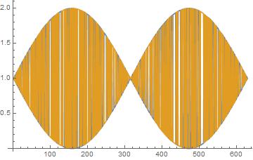
e5 = {e1, e2, e3, e4};
roots = Transpose[{e1, e2, e3, e4}];
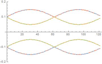
ListPlot[e5, PlotRange -> {-0.2, 0.2}]

enter image description here

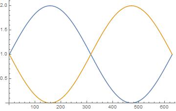
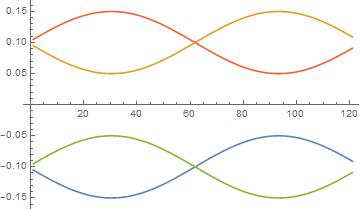
res = FoldList[permMatch, {{0, 0, 0, 0}, {0, 0, 0, 0}}, roots] // Rest;
finalResult = Map[(# // First) &, res] // Transpose;
finalResult // ListLinePlot

enter image description here

EDIT (last one, I promise)

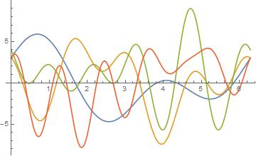
Tried this on a much messier problem

f1 = Sin[t] + 3 Cos[t] + 3 Sin[2 t]
f2 = 2 Sin[t] + 3 Cos[4 t] - 3 Sin[2 t]
f3 = 2 Sin[3 t] + 3 Cos[4 t] - 3 Sin[5 t] + 1
f4 = 2 Sin[6 t] + 3 Cos[5 t] - 3 Sin[t]

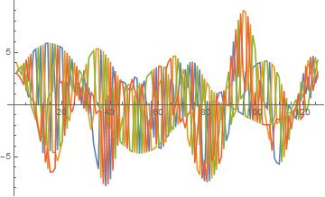
enter image description here

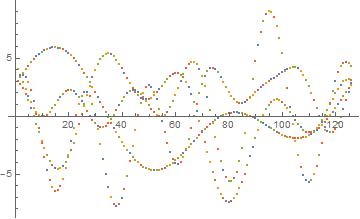
Now scramble it all up.

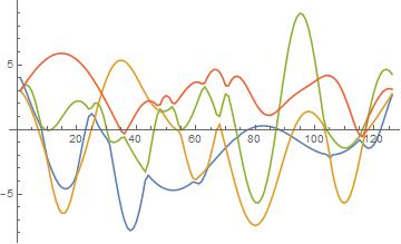
    scrambled = Table[{f1, f2, f3, f4}[[RandomSample[Range[4]]]], {t, 0, 2π, .05}]

enter image description here enter image description here

When I ran the algorithm...

enter image description here

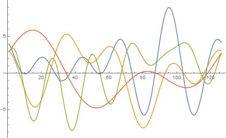
Not a right match. Needed to weight the derivative portion more, and now it works out.

WEIGHT = 10;    

permMatchWeight[{vals_, dels_}, l2_] := 
 Module[{l1 = {vals, dels}, ps, bestPerm}, 
  ps = Map[({#, WEIGHT (# - vals)}) &, Permutations[l2]];
  bestPerm = Sort[ps, Norm[l1 - #1] < Norm[l1 - #2] &] // First]

enter image description here

$\endgroup$
4
  • 1
    $\begingroup$ Your code is very handy. It should be implemented in next version of Mathematica. I run simulation for various input parameters, and it was working smoothly for up two 4 roots. Furthermore, I ensured that roots are Real. But when I run with 8 roots, it runs indefinitely. I added zeros where it should be. Is slowness due to permutations? Or should I add something to correct for number of roots I wondered if your code can be parallelized? $\endgroup$
    – Aschoolar
    Commented Jul 6, 2017 at 0:50
  • $\begingroup$ ,Is there something that I should look out when using your code. Like input requirements etc. $\endgroup$
    – Aschoolar
    Commented Jul 6, 2017 at 1:19
  • 1
    $\begingroup$ I'm guessing it is slow due to permutations, as with 8 roots, you have 8! Permutations to look through. Brute force method. I'll fiddle with it, I am sure it can be streamlined. $\endgroup$
    – MikeY
    Commented Jul 6, 2017 at 3:02
  • $\begingroup$ 8! That is too much. I will have to avoid condition to run into it....There is also another condition to avoid. Sometimes one scrambled pair of sine is shorter in length than the other scrambler pair. $\endgroup$
    – Aschoolar
    Commented Jul 8, 2017 at 19:53
3
$\begingroup$

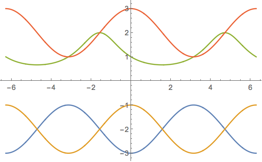
A standard way to solve an equation $f(x,y)=0$ for the function $y(x)$ satisfying a condition $y(x_0)=y_0$ is to integrate the differentiated equation as an IVP: $$f_x(x,y) + f_y(x,y)\,y' = 0,\quad y(x_0) = y_0$$ This will work on equations with multiple solutions as long as the solution functions do not cross or touch each other. If there are such singular points, then one may "blow up" the singularity by differentiating the equation further and using the derivatives of $y(x)$ to separate the solutions. Simple crossings may be resolved by differentiating once. The resulting differential equation is second-order, and the dependent variables $\langle y(x),\,y'(x)\rangle$ will be distinct for distinct solutions. For solutions that are tangent, higher-order derivatives would be needed depending on the order of tangency.

eqn = (y - Cos[x] + 2) (y + Cos[x] + 2) (y - Cos[x] - 2) (2 y + Sin[x] y - 2) == 0;
eqnx = eqn /. y -> y[x];  (* equation with y as a function of x *)
ode1 = D[eqnx, x];        (* first-order ODE *)
ode2 = D[ode1, x];        (* second-order ODE *)

ics0 = NSolve[eqnx /. x -> -2 Pi, y[-2 Pi]];
ics1 = First@Solve[ode1, y'[x]] /. x -> -2 Pi /. ics0;
ics = Apply[Equal, Join[ics0, ics1, 2], {2}]
(*
{{y[-2 \[Pi]] == -3., Derivative[1][y][-2 \[Pi]] == 0.},
 {y[-2 \[Pi]] == -1., Derivative[1][y][-2 \[Pi]] == 0.},
 {y[-2 \[Pi]] == 1., Derivative[1][y][-2 \[Pi]] == -0.5},
 {y[-2 \[Pi]] == 3., Derivative[1][y][-2 \[Pi]] == 0.}}
*)

NDSolveValue[{ode2, #}, y, {x, -2 Pi, 2 Pi}, 
    Method -> {"FixedStep", 
      Method -> {"Projection", "Invariants" -> ({eqnx, ode1} /. Equal -> Subtract)}}, 
    StartingStepSize -> 1/100] & /@ ics // ListLinePlot

enter image description here

Remark on robustness: One should note that I used a "FixedStep" method, together with the "Projection" method. The projection method projects the solution step back onto the original equations, basically using Newton's method. This ensures the accuracy of the steps. However, Newton's method tends not to work well near the singular points, that is, the crossings. The fixed-step method was used to step over the crossings and avoid the numerical difficulties they present. With adaptive step-size methods, the step size tends to diminish near the crossings and trouble is encountered. Also, the wrong StartingStepSize, such as 2 Pi/100 in this example, leads to a step landing on a singularity and fails. Some adjustment may be necessary in some problems.

$\endgroup$

Your Answer

By clicking “Post Your Answer”, you agree to our terms of service and acknowledge you have read our privacy policy.

Not the answer you're looking for? Browse other questions tagged or ask your own question.