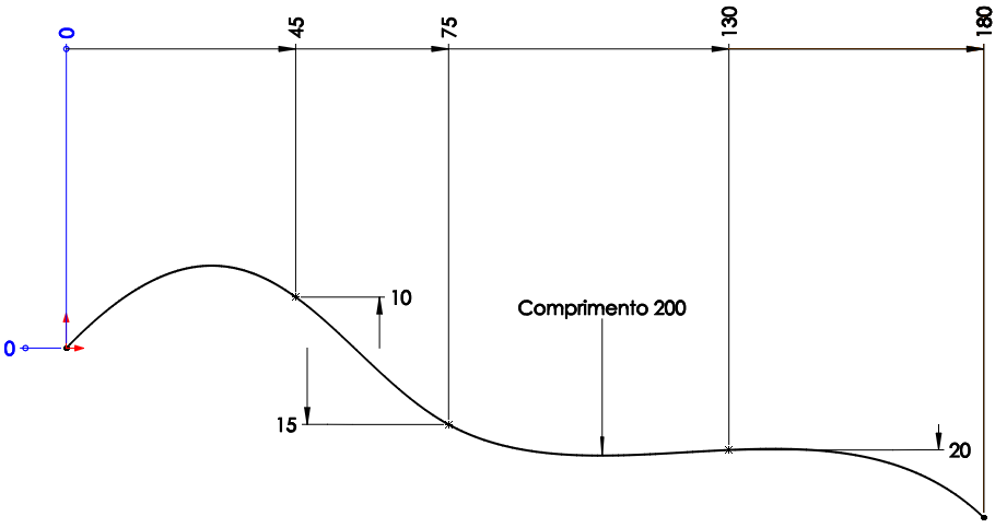
Assuming solving for the final y-coordinate is sought, which is what it sounds like:
len[y_?NumericQ] :=
 With[{spl = Interpolation[
    {{0, 0}, {45, 10}, {75, -15}, {130, -20}, {180, y}},
    Method -> "Spline"]},
  NIntegrate[Sqrt[1 + spl'[t]^2], {t, 0, 180}]]
Check OP's solution
len[-33.25904873]
(*  205.858  *)
Try to find a better one:
FindRoot[len[y] == 200, {y, 0}]
len[y] /. %
FindRoot::lstol: The line search decreased the step size to within tolerance specified by AccuracyGoal and PrecisionGoal but was unable to find a sufficient decrease in the merit function.... >>
(*
  {y -> -15.8953}
  202.674
*)
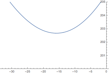
The answer to question 2 is that, yes, there could be more than one solution, but, in fact, there is not even one:
Plot[len[y], {y, -33, 0},
 GridLines -> {None, {200}},  PlotRange -> {200, 205}]

Update --
Here's the B-spline example from the docs (pointed out by the OP) adapted to the OP's problem. It still shows it is impossible. Someone either will have to guess the correct basis, or perhaps the OP can find a suitable one.
ClearAll[len];
bs[y_?NumericQ] := Module[{pts, dist, param, knots, m, ctrlpts},
   pts = {{0, 0}, {45, 10}, {75, -15}, {130, -20}, {180, y}};
   dist =
    Accumulate[
     Table[EuclideanDistance[pts[[i]], pts[[i + 1]]], {i, Length[pts] - 1}]];
   param = N[Prepend[dist/Last[dist], 0]];
   knots = {0, 0, 0, 0, 1/3, 2/3, 1, 1, 1, 1};
   m = Table[
     BSplineBasis[{3, knots}, j - 1, param[[i]]], {i, Length@param}, {j, 6}];
   ctrlpts = LinearSolve[m, pts];
   BSplineFunction[ctrlpts]
   ];
len[y_?NumericQ] := NIntegrate[Norm[D[bs[y][t], t]], {t, 0, 1}];
Solution:
splsol = FindRoot[len[y] == 200, {{y, 0}}]
len[y] /. splsol
(*
  {y -> -17.3114}
  201.19
*)


