0
$\begingroup$

I would like to interpolate a data set which represents a curve of an empirical cumulative distribution function (CDF). Hence, the y entries are between 0 and 1, continuous and non-decreasing, and at the extremities, must equal 0 on the left, 1 on the right with a derivative tending to zero.

An example of data is

data=
{
  {406.833, 0.05}, {423.458, 0.1}, {436.375, 0.15}, {448.042, 0.2}, 
  {459.583, 0.25}, {467.75, 0.3}, {479.083, 0.35}, {489.917, 0.4},
  {500.875, 0.45}, {508.542, 0.5}, {521.792, 0.55}, {536.75, 0.6}, 
  {547.458, 0.65}, {560.667, 0.7}, {584.208, 0.75}, {598.583, 0.8}, 
  {632.875, 0.85}, {672.583, 0.9}, {726.542, 0.95}
}

The first element of any pair is a value of the $x$ variate; the second element is the cumulative probability $Pr(X \leq x)$. Hence, the second element starts near zero, ends near 1, and is continously non-decreasing in between.

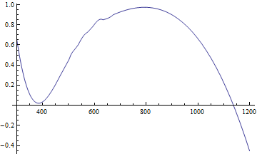
Using Interpolation[data], I can plot the estimated function, but it behaves improperly for a CDF as soon as I use a too small x or a too large x. For example,

enter image description here

which goes up above 0 before 400, and plunges below 1 (and even negative) after 800.

How can I impose constraints so the interpolation function has the behavior of a CDF?

$\endgroup$
1

1 Answer 1

2
$\begingroup$

Fit your data to a CDF using NonlinearModelFit

data = {{406.833, 0.05}, {423.458, 0.1}, {436.375, 0.15}, {448.042, 
    0.2}, {459.583, 0.25}, {467.75, 0.3}, {479.083, 0.35}, {489.917, 
    0.4}, {500.875, 0.45}, {508.542, 0.5}, {521.792, 0.55}, {536.75, 
    0.6}, {547.458, 0.65}, {560.667, 0.7}, {584.208, 0.75}, {598.583, 
    0.8}, {632.875, 0.85}, {672.583, 0.9}, {726.542, 0.95}};

Select a distribution to fit, e.g., LogNormalDistribution

Clear[nlm];
nlm = NonlinearModelFit[data, CDF[LogNormalDistribution[m, s], x], {m, s}, x];

The parameters in the fitted model are

param = nlm["BestFitParameters"]

(*  {m -> 6.2435, s -> 0.173715}  *)

The estimate for the CDF is

nlm // Normal

enter image description here

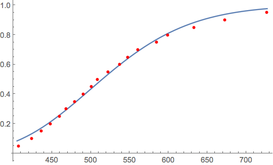
Plot[nlm[x], {x, 405, 727},
 Epilog -> {Red, AbsolutePointSize[4], Point[data]}]

enter image description here

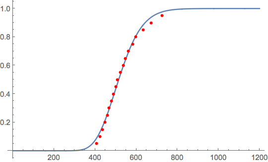
A CDF has the expected behavior at the extremes.

Plot[nlm[x], {x, 0, 1200},
 Epilog -> {Red, AbsolutePointSize[4], Point[data]}]

enter image description here

$\endgroup$
2
  • $\begingroup$ Thanks for the suggestion, but I need a non-parametric solution. $\endgroup$ Commented Jun 24, 2016 at 11:24
  • $\begingroup$ Bob Hanlon's solution is not really a parametric solution ... It is just using an arbitrary structure to assist the fit. I think it is quite clever. And yes - you will get different results based on different distributions ... but that is no different to getting different results using different optimisation algorithms, or different numerical starting points, etc ... Ultimately, the end result is vastly better than what you started with. $\endgroup$
    – wolfies
    Commented Jun 24, 2016 at 17:48

Your Answer

By clicking “Post Your Answer”, you agree to our terms of service and acknowledge you have read our privacy policy.

Not the answer you're looking for? Browse other questions tagged or ask your own question.