This is two sums, which are similar, but the first is good practice for the second (and the $\beta_{0k}$s are a little different from the ones with $n>0$).
Throughout, we make the following changes in notation, consistent with your intention to treat $qa$ as the ordinate for plotting and the other two combinations as parameters:
- $qa \rightarrow x \text{ and }$
x,
- $D\Delta / a^2 \rightarrow \delta \text{ and }$
DDeltaOverASquared, and
- $\overline{\rho} a / D \rightarrow r \text{ and }$
RhoAOverD.
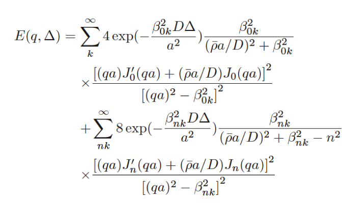
In this notation, the original sum is \begin{align}
\hat{E}(x; \delta, r) =
&\sum_{k=1}^{\infty} 4 \mathrm{e}^{-\beta_{0k}\delta}\frac{\beta_{0k}^2}{r^2 + \beta_{0k}^2 \phantom{{}-n^2}} \frac{(x J_0'(x) + r J_0(x))^2}{(x^2 - \beta_{0k}^2)^2} \\
+
\sum_{n=1}^\infty & \sum_{k=1}^\infty 8 \mathrm{e}^{-\beta_{nk}\delta}\frac{\beta_{nk}^2}{r^2 + \beta_{nk}^2 - n^2} \frac{(x J_n'(x) + r J_n(x))^2}{(x^2 - \beta_{nk}^2)^2}
\end{align}
Facts about $\beta_{nk}$
For each $n$, $\beta_{nk}$ is a strictly monotonically increasing function of $k$. For very large $x$, $J_n(x) \approx \sqrt{\frac{2}{\pi x}} \cos \left( x - \frac{n \pi}{2} - \frac{\pi}{4} \right)$.
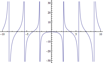
For $n=0$ and large $\beta$, we consider $ f(\beta) = \frac{J_0'(\beta)}{J_0(\beta)} = -\beta \frac{J_1(\beta)}{J_0(\beta)}$ using the cosine formula above, and see that $f(\beta)$ has a zero at local minima and maxima of $J_0(\beta)$ and has a vertical asymptote at zeroes of $J_0(\beta)$, and the zeroes and asymptotes are interleaved. With some effort, we can show that this function is strictly monotonically decreasing between the vertical asymptotes on $(0,\infty)$. Since $0 \cdot f(0) = 0$, the zeroes of $f$ (equivalently, the zeroes of $J_1$) partition $[0,\infty)$ into intervals each of which is injectively mapped to $(\Bbb{R} \setminus \{0\})$ (ignoring the asymptote, since we assume $r$ is finite). The first few zeroes of $\beta f(\beta)$ are $\beta = 0$ and
NSolve[{-β (BesselJ[1, β]/BesselJ[0, β]) == 0, 1 < β < 14}, β]
(*  {{β -> 3.83171}, {β -> 7.01559}, {β -> 10.1735}, {β -> 13.3237}}  *)
the last two of which already differ by only $3.15...$ and the difference between subsequent zeroes gets closer and closer to $\pi$, the spacing between the zeroes of sine (the derivative of the cosine in the asymptotic formula). Our takeaway from this is $$ (k-1)\pi \leq \beta_{0k} $$ and we will use this estimate to bound the error in truncating the first sum. We package the above into a machine which can find these $\beta$s:
Clear[B];
B[0, 1, 0, opts___] = 0;
B[0, k_ /; k > 1, 0, opts___] := BesselJZero[1, k - 1];
B[0, k_ /; k >= 1, RhoAOverD_ /; RhoAOverD > 0, opts___] :=
  z /. FindRoot[
    -z^2 BesselJ[1, z]/BesselJ[0, z] == -RhoAOverD,
    {z,
      If[k > 1, BesselJZero[1, k - 1], 0] + 1,
      If[k > 1, BesselJZero[1, k - 1], 0],
      BesselJZero[1, k]
  }, opts];
B[0, k_ /; k >= 1, RhoAOverD_ /; RhoAOverD < 0, opts___] :=
  z /. FindRoot[
    -z^2 BesselJ[1, z]/BesselJ[0, z] == -RhoAOverD,
    {z,
      BesselJZero[1, k] - 1,
      If[k > 1, BesselJZero[1, k - 1], 0],
      BesselJZero[1, k]
  }, opts];
We handle the first zero specially because FindRoot[] seems to have some difficulty locating the double root at zero. Also, since every one of our partitions of $(0,\infty)$ has an asymptote in it, we search for positive values of $r$ on one side of the asymptote and for negative values on the other side. The partitions are at least $\pi$ units wide, so backing into the partition by $1$ unit from the end (on the side of the asymptote where we expect to find the solution) is safe. Since the zeroes of the function are on the borders of two partitions, they're called out specially too (also since the extra zero at zero causes the zeroes of this function to be offset by one from the zeroes of $J_1$). Finally, at some point, we may wish to improve the accuracy/precision of a $\beta$, so we can pass relevant options in to FindRoot[].
B[0, 1, 0]
B[0, 2, 0]
B[0, 1, 1]
B[0, 1, -1]
B[0, 1, 1, WorkingPrecision -> 30]
B[0, 1, -1, WorkingPrecision -> 35]

(*  0  *)
(*  BesselJZero[1,1]  *)
(*  1.17726  *)
(*  3.76181  *)
(*  1.17725649964807633454475810267  *)
(*  3.7618061255679366126466190513942089  *)
For $n>0$ and large $\beta$, we consider $ \beta f_n(\beta) = \beta \frac{J_n'(\beta)}{J_n(\beta)} = -n + \beta\frac{J_{n-1}(\beta)}{J_n(\beta)}$ and repeat our reasoning using the cosine formula above. This analysis is largely unchanged, except everything is shifted by $n$ units and there is a zero-free gap in $J_{n-1}(\beta)$, so the first partition is wider. Our estimates are \begin{align}
0 &\leq \beta_{n1} & n &\geq 1 \\
\frac{(n - 1) \pi}{2} + (k - 1)\pi = (2k + n -3)\frac{\pi}{2} &< \beta_{nk} & n &\geq 1, k > 1 \text{.}
\end{align}
And we use these observations to put together the rest of the gadgets we need to find the $\beta$s. The only significant change is the shift by $n$ and having to move the condition between RhoAOverD and n to the end of the definition (because n cannot be used in a Condition at the point that RhoAOverD is declared).
B[n_ /; n > 0, 1, RhoAOverD_, opts___] := 0  /; RhoAOverD == -n ;
B[n_ /; n > 0, k_ /; k > 1, RhoAOverD_, opts___] :=
  BesselJZero[1, k - 1]  /; RhoAOverD == -n ;
B[n_ /; n > 0, k_ /; k >= 1, RhoAOverD_, opts___] := (
  z /.
  FindRoot[-n + (z BesselJ[-1 + n, z])/BesselJ[n, z] == -RhoAOverD,
    {z,
      If[k > 1, BesselJZero[n - 1, k - 1], 0] + 1,
      If[k > 1, BesselJZero[n - 1, k - 1], 0],
      BesselJZero[n - 1, k]},
  opts])  /; RhoAOverD < -n ;
B[n_ /; n > 0, k_ /; k >= 1, RhoAOverD_, opts___] := (
  z /.
  FindRoot[-n + (z BesselJ[-1 + n, z])/BesselJ[n, z] == -RhoAOverD,
    {z,
      BesselJZero[n - 1, k] - 1,
      If[k > 1, BesselJZero[n - 1, k - 1], 0],
      BesselJZero[n - 1, k]},
  opts])  /; RhoAOverD > -n ;

B[1, 1, 0]
B[1, 2, 0]
B[1, 1, 1]
B[1, 1, -1]
B[1, 1, 1, WorkingPrecision -> 30]
B[1, 1, -1, WorkingPrecision -> 35]

(*  1.84118  *)
(*  5.33144  *)
(*  2.40483  *)
(*  0  *)
(*  2.40482555769577276862163187933  *)
(*  0  *)
(Note that 0 is already an infinite precision zero.)
As a future direction for improvement, starting the FindRoot searches one unit from the end of the interval containing the $\beta$s is not the best way to go. The asymptotic estimate for $J_n$ suggests we should use something vaguely like $\beta \tan \beta$, tweaked so its zero and asymptote match in the interval we are searching to get a starting estimate. This will likely make the FindRoot much quicker, especially for large $k$. However, solving this tangent equation will cost significantly more time, so instrumentation and testing are in order.
Aside
We actually have enough to plot something now.
summand0[x_, DDeltaOverASquared_, RhoAOverD_] =
  4 E^(-B[0, k, RhoAOverD] DDeltaOverASquared)
  B[0, k, RhoAOverD]^2/(RhoAOverD^2 + B[0, k, RhoAOverD]^2)
  (x D[BesselJ[0, x], x] + RhoAOverD BesselJ[0, x])^2/(x^2 - B[0, k, RhoAOverD]^2)^2
summandN[x_, DDeltaOverASquared_, RhoAOverD_] =
  8 E^(-B[n, k, RhoAOverD] DDeltaOverASquared)
  B[n, k, RhoAOverD]^2/(RhoAOverD^2 + B[n, k, RhoAOverD]^2 - n^2)
  (x D[BesselJ[n, x], x] + RhoAOverD BesselJ[n, x])^2/(x^2 - B[n, k, RhoAOverD]^2)^2

eHat10[x_, DDeltaOverASquared_, RhoAOverD_] =
  Sum[summand0[x, DDeltaOverASquared, RhoAOverD], {k, 1, 10}] +
  Sum[summandN[x, DDeltaOverASquared, RhoAOverD], {k, 1, 10}, {n, 1, 10}];
eHat11[x_, DDeltaOverASquared_, RhoAOverD_] =
  Sum[summand0[x, DDeltaOverASquared, RhoAOverD], {k, 1, 11}] +
  Sum[summandN[x, DDeltaOverASquared, RhoAOverD], {k, 1, 11}, {n, 1, 11}];


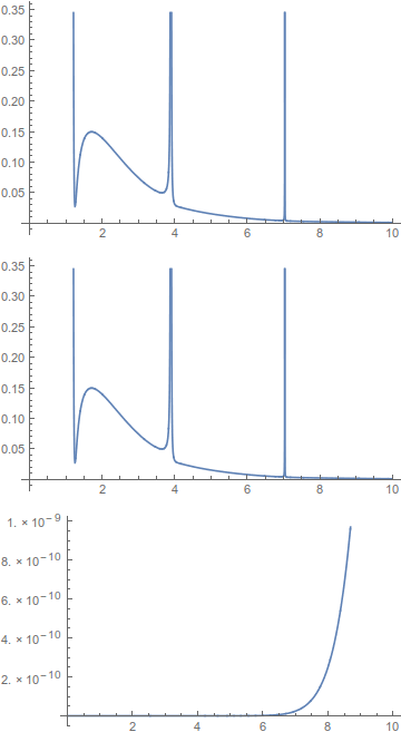
Plot[Evaluate[eHat10[x, 1, 1]], {x, 0, 10}]
Plot[Evaluate[eHat11[x, 1, 1]], {x, 0, 10}]
Plot[Evaluate[eHat11[x, 1, 1] - eHat10[x, 1, 1]], {x, 0, 10}]

These are just truncations to $110$ terms (eHat10) and $132$ terms (eHat11). They plot the same and differ by less than $\sim 10^{-9}$ over the plotted interval. So for parameters near $1$, the convergence is rather quick. We don't yet know that the rest of the terms don't eventually accumulate significant error, but we will find out that they do not for parameters near $1$.
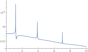
Given the large range of values appearing in the plots, a LogPlot might be more informative.
LogPlot[Evaluate[eHat11[x, 1, 1]], {x, 0, 10}, PlotRange -> All]

We use Evaluate[] in the plots so that the finite sums will be expanded and the $\beta$s evaluated once and the resulting rational expressions used repeatedly. This is much faster than repeating the calculation of the $\beta$s every time Plot evaluates its first argument. (Don't try to FullSimplify in this Evaluate call. The kernel will spend more time trying to simplify, without much effect, than it does plotting without simplifying.)
This might be enough to tell you everything you want to know. But generally, we need confidence that the truncated sums are actually close to the infinite sums and have some bound on the discrepancy. Let's get those error estimates and make some functions that give us values with bounds.
The first sum
Now we analyze $$
S_0(K) = \sum_{k=K+1}^{\infty} 4 \mathrm{e}^{-\beta_{0k}\delta}\frac{\beta_{0k}^2}{r^2 + \beta_{0k}^2 \phantom{{}-n^2}} \frac{(x J_0'(x) + r J_0(x))^2}{(x^2 - \beta_{0k}^2)^2}
$$ to estimate the error in truncating the first sum after $K$ terms. From the above, $$ \mathrm{e}^{- \beta_{0k} \delta} \leq \mathrm{e}^{-(k-1)\pi \delta} \text{.} $$ We could fuss with the fraction in $\beta$, but it is sufficient to estimate it with $$ \frac{\beta_{0k}^2}{r^2 + \beta_{0k}^2} \leq 1 \text{.} $$ Further, both $J_0$ and $J_0'$ are bounded by $1$, so for $\beta_{0k} > (k-1)\pi > \sqrt{2}x$, $$
\frac{(x J_0'(x) + r J_0(x))^2}{(x^2 - \beta_{0k}^2)^2}
= \frac{(x J_0'(x) + r J_0(x))^2}{(\beta_{0k}^2 - x^2)^2}
\leq \frac{(x J_0'(x) + r J_0(x))^2}{x^4}
\leq \frac{(|x| + |r|)^2}{x^4} \text{.}
$$ This gives us our first indication of a lower bound on $K$ : $$ K > \frac{\sqrt{2}}{\pi} x \text{.} $$ Putting these together, we have $$
S_0(K) \leq \sum_{k=K+1}^{\infty} 4 \mathrm{e}^{-(k-1)\pi \delta}\cdot 1 \cdot \frac{(|x| + |r|)^2}{x^4} \qquad\qquad [ K > \frac{\sqrt{2}}{\pi} x ] \text{.} $$
Pulling out everything not depending on $k$, we are left with a simple geometric series: $$
S_0(K) \leq 4 \frac{(|x| + |r|)^2}{x^4} \sum_{k=K+1}^{\infty} \mathrm{e}^{-(k-1)\pi \delta} = 4 \frac{(|x| + |r|)^2}{x^4} \frac{\mathrm{e}^{(1-K)\pi \delta}}{\mathrm{e}^{\pi \delta} - 1} \qquad\qquad [ K > \frac{\sqrt{2}}{\pi} x ] \text{.} $$
Of course, we can make this sum as small as we like by increasing $K$. (Happily, this error estimate gets smaller as $x$ increases, starting once $x \approx \sqrt{r}$, so we do not have to take longer and longer sums as $x$ increases.)
(We could do better. The same sorts of estimates for the $\beta$s could be turned into upper bounds, which would give us a lower bound for the sum $S_0(K)$. This lower bound would be of about the same shape as the estimate we have, it would just skip a few terms. Once the lower bound and upper bound agreed sufficiently, we could stop increasing $K$. This would happen earlier than the method we are currently using, taking $0$ as the lower bound.)
Let's capture this in code
summand0[x_, DDeltaOverASquared_, RhoAOverD_] =
  4 E^(-B[0, k, RhoAOverD] DDeltaOverASquared)
  B[0, k, RhoAOverD]^2/(RhoAOverD^2 + B[0, k, RhoAOverD]^2)
  (x D[BesselJ[0, x], x] + RhoAOverD BesselJ[0, x])^2/(x^2 - B[0, k, RhoAOverD]^2)^2
sum0K[K_, x_, DDeltaOverASquared_, RhoAOverD_] :=
  Sum[summand0[x, \[Delta], r], {k, 1, K}]
sum0Error[K_, x_, DDeltaOverASquared_, RhoAOverD_] :=
  4 (Abs[x] + Abs[RhoAOverD])^2/x^4
  E^((1 - K) Pi DDeltaOverASquared)/(E^(Pi DDeltaOverASquared) - 1)
And let's see what the error does versus $x$.
LogPlot[sum0Error[3, x, 1, 1], {x, 0, 10}]
... and we find the error is nicely shrinking as $x$ increases.
The second sum
There's an easy way to find cutoffs for double sums and a tricky way that generally uses half as many terms. The easy way is to find upper bounds $N$ and $K$ and sum on the rectangle $(n,k) \in [1,N]\times[1,K]$. A slightly smarter way is to find a line in the $N$-$K$ plane and only sum the terms bounded by the axes and this line. As a gross generalization, this line typically runs along the diagonal of the rectangle. I'm a little lazy (although maybe that's not obvious given the length of this answer and the endless stream of parenthetical comments), so I'll go with the two cutoffs.
Sadly, it's not quite as simple as that. We don't have shrinking bounds on the $\beta_{n1}$s because they could be in the interval prior to the first asymptote, which means we only know they're greater than or equal to zero. We'll have to handle $k=1$ separately, but the above comments about cutoffs $N$ and $K$ hold for the $\sum_{k=2}^K \dots$ sums.
We wish to study these sums to estimate the truncation error. For $K >1$, \begin{align}
S_K(N,K) &= \sum_{n=1}^{N} \sum_{k=K+1}^\infty 8 \mathrm{e}^{-\beta_{nk}\delta}\frac{\beta_{nk}^2}{r^2 + \beta_{nk}^2 - n^2} \frac{(x J_n'(x) + r J_n(x))^2}{(x^2 - \beta_{nk}^2)^2} \text{,} \\
S_N(N) &= \sum_{n=N+1}^\infty \sum_{k=2}^\infty 8 \mathrm{e}^{-\beta_{nk}\delta}\frac{\beta_{nk}^2}{r^2 + \beta_{nk}^2 - n^2} \frac{(x J_n'(x) + r J_n(x))^2}{(x^2 - \beta_{nk}^2)^2} \text{, and } \\
S_1(N_1) &= \sum_{n=N_1+1}^\infty 8 \mathrm{e}^{-\beta_{n1}\delta}\frac{\beta_{n1}^2}{r^2 + \beta_{n1}^2 - n^2} \frac{(x J_n'(x) + r J_n(x))^2}{(x^2 - \beta_{n1}^2)^2} \text{.}
\end{align}
The first two we analyze as for the first sum: \begin{align}
\mathrm{e}^{-\beta_{nk} \delta} &\leq \mathrm{e}^{(2k+n-3)\pi \delta/2} \text{,} \\
\frac{\beta_{nk}^2}{r^2 + \beta_{nk}^2 - n^2} &\leq \frac{\pi^2}{\pi^2 - 4} \text{, and} \\
\frac{(x J_n'(x) + r J_n(x))^2}{(x^2 - \beta_{nk}^2)^2} &\leq \frac{|x| + |r|}{x^4} & &[K \geq \frac{3-n}{2} + \frac{\sqrt{2}}{\pi} x \geq 1 + \frac{\sqrt{2}}{\pi} x ] \text{.}
\end{align}
As before, we used the lower bound on the $\beta$s for the exponential and the exact same estimating for the Bessel functions fraction. The fraction in $\beta$s is a little trickier. Note that as $n$ increases to $r$, the ratio increases to approximately $1$. Subsequently, the $\beta$s increase by a bit more than $\pi/2$ (asymptotically decreasing to $\pi/2$) every time $n$ increases by $1$ or by a bit more than $\pi$ (asymptotically decreasing ot $\pi$) every time $k$ increases by $1$. Looking at $\lim_{k \rightarrow \infty} \frac{(\beta + k \alpha \pi)^2}{r^2 + (\beta + k \alpha \pi)^2 - (r+k)^2} = \frac{\pi^2}{\pi^2 - (1/\alpha)^2}$, which is maximized for $\alpha \in [1/2,\infty)$ by $\alpha = 1/2$, we find that $\frac{\pi^2}{\pi^2 - 4}$ is a bound we can use. Then summing the geometric series, we have \begin{align}
S_K(N,K) &\leq \frac{8 \pi^2}{\pi^2 - 4} \frac{|x| + |r|}{x^4} \frac{\mathrm{e}^{-(N+2K-3)\delta \pi/2} \left( \mathrm{e}^{N \delta \pi / 2} - 1 \right)}{ \left( \mathrm{e}^{\delta \pi / 2} - 1 \right)^2 \left( \mathrm{e}^{\delta \pi/2} + 1 \right)} & &[K \geq 1 + \frac{\sqrt{2}}{\pi} x] \\
S_N(N) &\leq \frac{8 \pi^2}{\pi^2 - 4} \frac{|x| + |r|}{x^4} \frac{\mathrm{e}^{-(N-1) \delta \pi / 2}}{\left( \mathrm{e}^{\delta \pi / 2} - 1 \right)^2 \left( \mathrm{e}^{\delta \pi/2} + 1 \right)} & &[K \geq 1 + \frac{\sqrt{2}}{\pi} x] \text{.}
\end{align}
 Where $ \beta _{nk} $ is defined by the transcendental equation:
