NDSolve for a system of nonlinear coupled pde

Question

I try to solve a system($n$) of coupled nonlinear 1-d PDE's which is basically coupled sine-Gordon equations (through 2nd spatial derivative) in time and space. I am interested in the dynamics when I increase the force gradually. So I use the final answer of smaller force $\beta$ and use it as initial condition for a larger force $\beta$. I wrote a code for smaller force and it produces the result in a decent amount of time (depending on the $n$). I use the final result as initial condition in the second part of my code. Since both parts of my code contain basically the same type of equations and only different in initial conditions and force magnitude, I expect it to run the same way as the first part. But, unfortunately no matter what I tried, the second part takes very long time and runs forever. Here is my code:

n = 3; η = 0.1; β = 0.4; L = 10; T = 100; τ = T/10;
af = Array[f, n];
txaf[x_, t_] := Through[af[x, t]];
eqs = Join[
Array[D[f[#][x, t], t, t] + η D[f[#][x, t], t] - 
  D[Sum[i f[i][x, t], {i, 1, #}] + #*Sum[f[j][x, t], {j, # + 1, n}], x, x] + 
  Sin[f[#][x, t]] - β Tanh[t/τ] == 0 &,n]]; 
init = {Union[Thread[Drop[txaf[x, 0], {(n + 1)/2}] == 
 0], {txaf[x, 0][[(n + 1)/2]] == 4 ArcTan[Exp[x]]}], 
Thread[Derivative[0, 1][txaf][x, 0] == 0]}; 
bc = {Thread[Derivative[1, 0][txaf][-L, t] == 0], 
Thread[Derivative[1, 0][txaf][L, t] == 0]};
sol = NDSolve[{eqs, init, bc}, af, {x, -L, L}, {t, 0, T}, 
MaxStepSize -> 0.05]

using as intial condition:

f0[x_] := Thread[First[Evaluate[txaf[x, T] /. sol]]];
df0[x_] := Thread[First[Evaluate[Derivative[0, 1][txaf][x, T] /. sol]]];

second part of my code:

Clear[af, eqs, init, bc]
β2 = 0.5;
af = Array[f, n];
txaf[x_, t_] =.;
txaf[x_, t_] := Through[af[x, t]];
eqs = Join[
Array[D[f[#][x, t], t, t] + η D[f[#][x, t], t] - 
  D[Sum[i f[i][x, t], {i, 1, #}] + #*Sum[f[j][x, t], {j, # + 1, n}], x, x] + 
  Sin[f[#][x, t]] - β - (β2 - β)*
   Tanh[t/τ] == 0 &, n]]; 
init = {Thread[txaf[x, 0] == f0[x]], 
Thread[Derivative[0, 1][txaf][x, 0] == df0[x]]}; 
bc = {Thread[Derivative[1, 0][txaf][-L, t] == 0], 
Thread[Derivative[1, 0][txaf][L, t] == 0]};
sol2 = NDSolve[{eqs, init, bc}, af, {x, -L, L}, {t, 0, T}, 
Method -> {"MethodOfLines", "SpatialDiscretization" -> {"TensorProductGrid", 
  "MaxPoints" -> 1000, "MinPoints" -> 500, "DifferenceOrder" -> "Pseudospectral"}}]

you can copy and paste the code and just hit the run. In the mean time if you have any comment to make the code more efficient for higher number of $n$, it would be greatly appreciated.

Answer 1

As noted in the question, the first code segment does run to completion. However, NDSolve also issues two warning messages.

NDSolve::ibcinc: Warning: boundary and initial conditions are inconsistent. >>

NDSolve::eerr: Warning: scaled local spatial error estimate of 37.88105237757757 at t = 100. in the direction of independent variable x is much greater than the prescribed error tolerance... >>

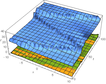
The first of these is due to the fact that init/.x -> L (or -L) does not match bc/.t -> 0. Correcting this should be straightforward. How serious the second warning is can be estimated from a plot of the solution.

Plot3D[Evaluate[Through[af[x, t]] /. Flatten@sol], {x, -L, L}, {t, 0, T}, 
    AxesLabel -> {x, t, f}]

which does not show obvious signs of numerical instability but, nonetheless, may not be as accurate as desired.

Not surprisingly, the second calculation also flags initial and boundary conditions as inconsistent. Additionally, it warns,

NDSolve::mxsst: Using maximum number of grid points 1000 allowed by the MaxPoints or MinStepSize options for independent variable x. >>

As noted in the question, the calculation is exceedingly slow. In fact, several minutes are required to reach t == 1. This is due to the Method choice, "DifferenceOrder" -> "Pseudospectral", which works best for periodic boundary conditions. Simply deleting this option greatly decreases runtime, but still requires a great deal of memory. To overcome this latter problem, one can reduce MaxPoints to 500, so that NDSolve becomes

sol2 = NDSolve[{eqs, init, bc}, af, {x, -L, L}, {t, 0, 100}, Method -> {"MethodOfLines",
    "SpatialDiscretization" -> {"TensorProductGrid", "MaxPoints" -> 500}}]

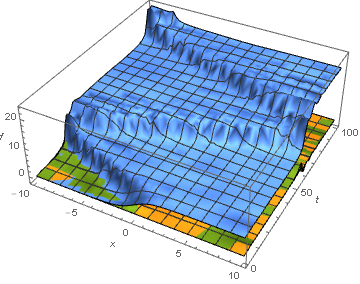
which, after several minutes produces an answer similar to that from the first computation.

Plot3D[Evaluate[Through[af[x, t]] /. Flatten@sol2], {x, -L, L}, {t, 0, T}, 
    AxesLabel -> {x, t, f}]

In summary, modifications to the options used by NDSolve lead to results in a reasonable amount of time. However, as noted above, the initial and boundary conditions should be modified so that init and bc are consistent at {L, 0} and {-L, 0). This, in itself, may improve the accuracy computations sufficiently to eliminate the second warnings.