P-values differ in tests for normality between Mathematica and SAS

Question

I am testing the following data for normality, in Mathematica and SAS:

data = {91.6667, 87.5, 54.1667, 75., 83.3333, 87.5, 83.3333, 62.5, 70.8333,70.8333, 75., 87.5, 66.6667, 87.5, 70.8333, 54.1667, 79.1667,95.8333, 70.8333, 37.5, 75., 79.1667, 75., 66.6667, 87.5, 75., 58.3333, 87.5, 91.6667, 91.6667, 54.1667, 87.5, 75., 79.1667, 95.8333, 66.6667, 91.6667, 62.5, 79.1667, 70.8333, 87.5, 91.6667, 54.1667, 87.5, 58.3333, 66.6667, 75., 83.3333, 70.8333, 58.3333, 75., 62.5, 41.6667, 37.5, 91.6667, 54.1667, 91.6667, 83.3333, 62.5, 87.5, 29.1667, 87.5, 91.6667, 75., 58.3333, 75.};

In Mathematica, my code is:

m = N[Mean[data]];
std = N[StandardDeviation[data]];
mo = Commonest[data][[1]];
Grid[{{Labeled[m, "Mean: ", Left]}, {Labeled[mo, "Mode: ", Left]}, {Labeled[std, "Standard Dev.: ", Left]}}, Alignment -> Left]
d = NormalDistribution[m, std];
H = DistributionFitTest[data, d, "HypothesisTestData"];
H["TestDataTable", All]

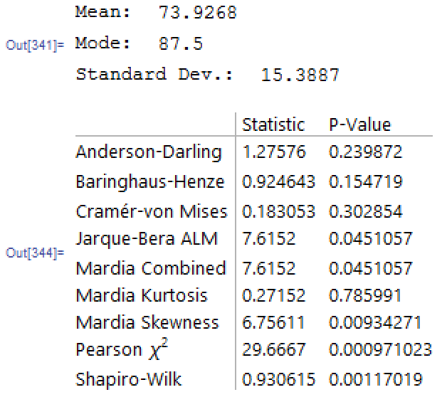
The output is:

In SAS, I'm using the Univariate procedure on the same data:

proc univariate data=knowledgescorescsv normal plots mu0=73.9268;
var Post;
run;

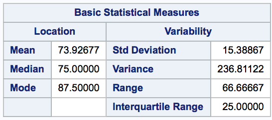
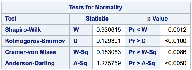
The output is:

As you can see, the mean, mode, standard deviation and Anderson-Darlin, Cramer-von Mises and Shapiro-Wilk statistics are the same in Mathematica and SAS. However, their corresponding p-values differ substantially, enough that Mathematica's p-values would lead me to fail to reject the null hypothesis while SAS p-values for these three statistics would lead me to reject the null hypothesis (i.e., that the data is normally distributed).

Why would the p-values for these statistics be so vastly different between Mathematica and SAS?

Answer 1

I should have looked at your code but I didn't, because I saw that the test-statistics for the tests in question were the same.

What I did then is to look up how p-values are computed for Anderson-Darling, which seems to be not as standardized as one might think. I came across this site where a formula is given to compute the p-value from the test-statistic. In your case, this formula was

p[ad_] := Exp[1.2937 - 5.709 ad + 0.0186 ad^2];
p[1.275759]
(* 0.00258163 *)

which supported the result that is given by SAS. At this point, I DID look on your code.

So what you do is to use the test wrong. By giving the (estimated) normal distribution as second parameter, Mathematica does not make the usual single sample normality test but it tests against your given distribution.

This results in the same statistic-value, but obviously the p-values are computed differently. Therefore, the simple solution is

DistributionFitTest[data, Automatic, {"TestDataTable", All}]

Answer 2

Yes, the P-values are being computed differently but there's a good reason for doing so and no bug report to Support needs to be made.

First generate some data:

SeedRandom[12345];
data = RandomVariate[NormalDistribution[], 2500];

Now test to see if the sample is from a normal distribution (and by that I mean any normal distribution: an unknown mean and unknown standard deviation):

h = DistributionFitTest[data, NormalDistribution[μ, σ], 
   "HypothesisTestData"];
h["TestDataTable", All]

$$ \begin{array}{l|ll} \text{} & \text{Statistic} & \text{P-Value} \\ \hline \text{Anderson-Darling} & 1.28718 & 0.00211436 \\ \text{Cramer-von Mises} & 0.184634 & 0.00785495 \\ \text{Pearson }\chi ^2 & 29.6667 & 0.000242055 \\ \text{Shapiro-Wilk} & 0.930615 & 0.0011702 \\ \end{array}$$

The same output is obtained with NormalDistribution[μ,σ] is replaced with Automatic.

But now suppose we wanted to test against a specific normal distribution. In fact suppose we test against a normal distribution with the same mean and standard deviation as the sample mean and sample standard deviation.

h = DistributionFitTest[data, 
   NormalDistribution[Mean[data], StandardDeviation[data]],
   "HypothesisTestData"];
h["TestDataTable", All]

$$\begin{array}{l|ll} \text{} & \text{Statistic} & \text{P-Value} \\ \hline \text{Anderson-Darling} & 1.27575 & 0.239873 \\ \text{Cramer-von Mises} & 0.183053 & 0.302856 \\ \text{Pearson }\chi ^2 & 29.6667 & 0.000971023 \\ \text{Shapiro-Wilk} & 0.930615 & 0.0011702 \\ \end{array}$$

So we see that all of the P-values (except the Shapiro-Wilk) have increased because we've stacked the deck by testing against a normal distribution with the same mean and standard deviation. In other words we're much less likely to reject the null hypothesis.

So the P-values differ but that's because we're testing two different hypotheses. The first is if the sample might have been drawn from an unspecified normal distribution and the other hypothesis deals with a specific normal distribution.

(I've only kept the tests that matched what SAS produced and why the Shapiro-Wilk P-value does not change is left as an exercise for the reader.)

Answer 3

Minor point: DistributionFitTest[myData, Automatic, {"TestDataTable", All}] blows up if myData includes negative numbers, but the fix is trivial:

DistributionFitTest[N[myData], Automatic, {"TestDataTable", All}]