22
$\begingroup$

I have a list of points in 3D, and I want to get a smooth interpolation or curve fit (it is more for illustration) of these points such that the first and second derivatives at the start and end points agree. With

ListInterpolation[pts1, {0, 1}, InterpolationOrder -> 4, PeriodicInterpolation -> True]

even the first derivatives do not agree.

$\endgroup$
3
  • 1
    $\begingroup$ Can you post your points somewhere, so that we can use them to compare? $\endgroup$
    – rcollyer
    Commented Sep 5, 2012 at 20:10
  • 7
    $\begingroup$ I might be understanding your question correctly, but if you want to ensure a continuous derivative you will need to use the following option: ListInterpolation[pts1, {0, 1}, InterpolationOrder -> 4,PeriodicInterpolation -> True, Method -> "Spline"]. By default ListInterpolation is using a Hermite interpolation which does not guarantee a continuous derivative. $\endgroup$
    – chuy
    Commented Sep 5, 2012 at 20:22
  • $\begingroup$ Is the function with open ends or a closed loop? And as @rcollyer already said, we really need the points. $\endgroup$ Commented Sep 5, 2012 at 21:16

2 Answers 2

26
$\begingroup$

It does seem that the options PeriodicInterpolation -> True and Method -> "Spline" are incompatible, so I'll give a method for implementing a genuine cubic periodic spline for curves. First, let's talk about parametrizing the curve.

Eugene Lee, in this paper, introduced what is known as centripetal parametrization that can be used when one wants to interpolate across an arbitrary curve in $\mathbb R^n$. Here's a Mathematica implementation of his method:

parametrizeCurve[pts_List, a : (_?NumericQ) : 1/2] /; MatrixQ[pts, NumericQ] := 
           FoldList[Plus, 0, Normalize[(Norm /@ Differences[pts])^a, Total]] 

The default setting of the second parameter for parametrizeCurve[] gives the centripetal parametrization. Other popular settings include a == 0 (uniform parametrization) and a == 1 (chord length parametrization).

Now we turn to generating the derivatives needed for periodic cubic spline interpolation. This is done through the solution of an appropriate cyclic tridiagonal system, for which the functions LinearSolve[], SparseArray[], and Band[] come in handy:

periodicSplineSlopes[pts_?MatrixQ] := 
 Module[{n = Length[pts], dy, ha, xa, ya}, {xa, ya} = Transpose[pts];
        ha = {##, #1} & @@ Differences[xa];
        dy = ({##, #1} & @@ Differences[ya])/ha;
        dy = LinearSolve[SparseArray[{Band[{2, 1}] -> Drop[ha, 2], 
                                      Band[{1, 1}] -> ListConvolve[{2, 2}, ha], 
                                      Band[{1, 2}] -> Drop[ha, -2],
                                      {1, n - 1} -> ha[[2]], {n - 1, 1} -> ha[[-2]]}], 
                         3 MapThread[Dot[#1, Reverse[#2]] &,
                                     Partition[#, 2, 1] & /@ {ha, dy}]];
        Prepend[dy, Last[dy]]]

Using Sjoerd's example:

sc = Table[{Sin[t], Cos[t], Cos[t] Sin[t]}, {t, 0, 2 π, π/5}] // N;
tvals = parametrizeCurve[sc]
   {0, 0.102805, 0.196242, 0.303758, 0.397195, 0.5, 0.602805, 0.696242,
    0.803758, 0.897195, 1.}

cmps = Transpose[sc];
slopes = periodicSplineSlopes[Transpose[{tvals, #}]] & /@ cmps;
{f1, f2, f3} = MapThread[Interpolation[Transpose[{List /@ tvals, #1, #2}], 
                                       InterpolationOrder -> 3, Method -> "Hermite",
                                       PeriodicInterpolation -> True] &,
                         {cmps, slopes}];

Plot the space curve:

Show[ParametricPlot3D[{f1[u], f2[u], f3[u]}, {u, 0, 1}],
     Graphics3D[{AbsolutePointSize[6], Point[sc]}]]
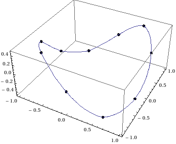
interpolated space curve

Individually plotting the components and their respective derivatives verify that the interpolating functions are $C^2$, as expected of a cubic spline:
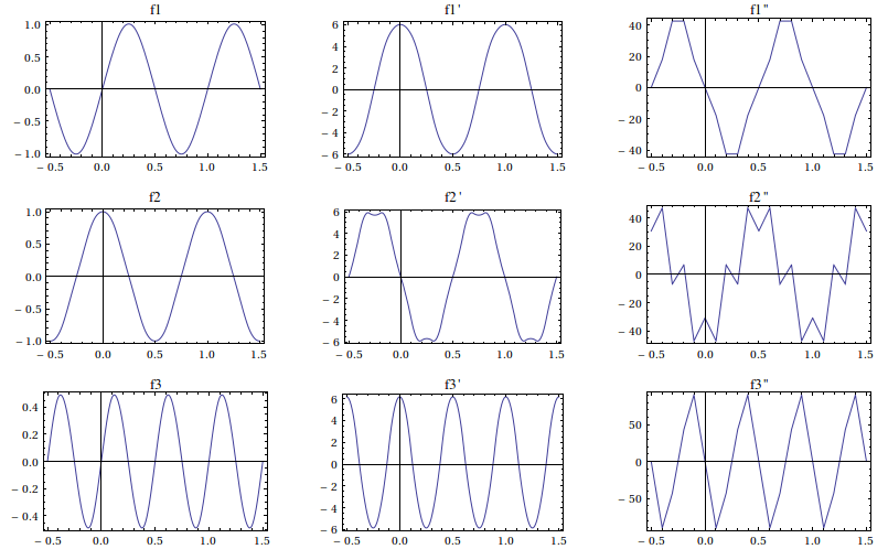
plots of components and derivatives

$\endgroup$
1
  • $\begingroup$ amazing!!! Thanks $\endgroup$
    – warsaga
    Commented Sep 6, 2012 at 10:33
15
$\begingroup$

You are talking about a list of 3D points and curve fitting. I therefore assume you want a function with a single parameter that describes a curve fitting through your set of points. I don't believe ListInterpolate can handle that.

My alternative is the following.

First, a set of 3D points:

pts1 = Table[{Sin[t], Cos[t], Cos[t] Sin[t]}, {t, 0, 2 \[Pi], \[Pi]/5}] // N;

I get incomprehensible errors (Interpolation::mspl: The Spline method could not be used because the data could not be coerced to machine real numbers) if I interpolate using the "Spline" method combined with PeriodicInterpolation. I therefore add the 2nd and 3rd point to the end of the array (the last and first one were already the same). This ensures a smooth connection of beginning and end of the list:

pts2 = Join[pts1, pts1[[2 ;; 3]]];

I now interpolate through each dimension separately:

f = Interpolation[#, InterpolationOrder->3, Method->"Spline"] & /@Transpose[pts2]

Plot the result:

p = Show[
      ParametricPlot3D[Through[f[x]], {x, 1, Length[pts1]}, Axes -> None],
      Graphics3D[{PointSize[0.02], Point@pts1}]
    ]

enter image description here

$\endgroup$
7
  • $\begingroup$ You are defining pts2 but you are not using it. $\endgroup$
    – Matariki
    Commented Sep 5, 2012 at 21:44
  • $\begingroup$ Showing the data points on the same plot would visually help ;-) $\endgroup$ Commented Sep 5, 2012 at 21:46
  • $\begingroup$ @VitaliyKaurov Something like the above? $\endgroup$ Commented Sep 5, 2012 at 21:53
  • $\begingroup$ @Matariki Copied the wrong version. Corrected, thanks. $\endgroup$ Commented Sep 5, 2012 at 21:56
  • $\begingroup$ Haha, yes, very neat :) +1 $\endgroup$ Commented Sep 5, 2012 at 21:56

Your Answer

By clicking “Post Your Answer”, you agree to our terms of service and acknowledge you have read our privacy policy.

Not the answer you're looking for? Browse other questions tagged or ask your own question.