Only final result from NDSolve

Question

Finally, I started to play with differential equations in Mathematica.

And I have faced the problem, which seems to me so basic that I'm afraid this question is going to be closed soon. However, I've failed in finding solution here or in the documentation center.

My question is: how to set that NDSolve will not save whole InterpolationFunction for the result?

I'm only interested in final coordinates or for example each 100th. Is there simple way to achieve that?

---

Anticipating questions:

• I know I can do something like r /@ Range[0.1, 1, .1] /. sol at the end, but still, there is whole interpolating function in memory. I want to avoid it because my final goal is to do N-Body simulation where N is huge and I will run out of the memory quite fast. What is important to me is only the set of coordinates as far in the future as it can be, not intermediate values.

• I can write something using Do or Nest but I want to avoid it since NDSolve allows us to implement different solving methods in handy way.

• I saw WolframDemonstrations/CollidingGalaxies and it seems there is an explicit code with Do :-/

• Another idea would be to put NDSolve into the loop but this seems to be not efficient. Could it be even compilable?

---

Just in case someone wants to show something, here is some sample code to play with:

G = 4 Pi^2 // N ;

sol = NDSolve[{
               r''[t] == -G r[t]/Norm[r[t]]^3,
               r[0] == {1, 0, 0},
               r'[0] == {0, 2 Pi // N, 0}
              },
              r,
              {t, 0, 1}, Method -> "ExplicitRungeKutta", MaxStepSize -> (1/365 // N)
             ]

 ParametricPlot3D[Evaluate[r[t] /. sol], {t, 0, 1}]

  (* Earth orbiting the Sun. Units: Year/AstronomicalUnit/SunMass 
     in order to express it simply*)

Answer 1

Here is a solution inspired from tutorial/NDSolveStateData (Mathematica 8):

G = 4 Pi^2 // N;

stateData = 
 First[
    NDSolve`ProcessEquations[
        {  r''[t] == -G r[t]/Norm[r[t]]^3, 
           r[0] == {1, 0, 0},
           r'[0] == {0, 2 Pi // N, 0}
           },
        r,
        {t, 0, 1}, 
         Method -> "ExplicitRungeKutta",
         MaxStepSize -> (1/365 // N)]]

res = Table[
  NDSolve`Iterate[stateData, i/365];
  rAndDerivativesValues = NDSolve`ProcessSolutions[stateData, "Forward"];
  stateData = First @ NDSolve`Reinitialize[stateData, Equal @@@ Most[rAndDerivativesValues]];
  rAndDerivativesValues,
  {i, 1, 365, 7 (* 7 = each week*)}
   ] ;

rAndDerivativesValues is the value of r[t] and its derivative at each week.
Example :

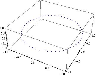
Here is one revolution of the Earth around the Sun :

ListPointPlot3D[#[[1, 2]] & /@ res ]

Answer 2

There is actually a somewhat cryptic but very simple way to make NDSolve only return the solution at the end point:

sol = NDSolve[{
    r''[t] == -G r[t]/Norm[r[t]]^3,
    r[0] == {1, 0, 0},
    r'[0] == {0, 2 Pi // N, 0}
  }, r, {t, 1, 1},
  Method -> "ExplicitRungeKutta", MaxStepSize -> (1/365 // N)
]

As it is easy to oversee: the difference is that you set the third argument to {t,1,1}, NDSolve will in such a case still start to solve from t=0 as that is where the initial conditions are given but it only returns the solution at the end point. That idea is of course much more useful when solving e.g. partial differential equations. If you compare the ByteCount of that solution you will find that it is indeed much smaller than that of thefull solution. It probably is interesting to note that it is also possible to use something like {t,0.9,1} to only get the solution for 0.9<=t<=1.

If you need the solution at only some points, you can also do something like:

fullsol = Reap[NDSolveValue[{
    r''[t] == -G r[t]/Norm[r[t]]^3,
    r[0] == {1, 0, 0},
    r'[0] == {0, 2 Pi // N, 0},
    WhenEvent[Mod[10*t, 1] == 0, Sow[{t, r[t]}]]
  }, r, {t, 1, 1},
  Method -> "ExplicitRungeKutta", MaxStepSize -> (1/365 // N)

]]

fullsol will then contain the accumulated solution points in a list which you can either convert to an interpolating function or use as it is for further investigations, e.g. visualizations:

Graphics3D[Point[fullsol[[2, 1, All, 2]]]]

You might want to test whether this or the NDSolve`Iterate approach does meet your needs better (it might well be that one is more performant than the other one for certain cases).

Answer 3

My question is: how to set that NDSolve will not save whole InterpolationFunction for the result?

There is actually a very simple way to do this: instead of specifying a list of functions in the second argument, specify an empty list instead. This now begs the question of how one can obtain results. The solution is to use the event location functionality of Mathematica, by trapping the required events with Sow[]/Reap[].

In the current Mathematica, one will of course use WhenEvent[]. As I do not have a newer version on the machine I am currently borrowing, I will use the older Method setting "EventLocator"; translation to the modern form ought to be straightforward, however.

First, the easy case of returning only the value at the endpoint:

G = 4 Pi^2 // N; 
Reap[NDSolve[{r''[t] == -G r[t]/Norm[r[t]]^3,
              r[0] == {1, 0, 0}, r'[0] == {0, 2 Pi, 0}},
             {}, (* empty! *) {t, 1}, 
             Method -> {"EventLocator", "Event" -> (t == 1), 
                        "EventAction" :> Sow[r[t]],
                        Method -> "ExplicitRungeKutta"}, 
             MaxStepSize -> 1/365]][[-1, 1, 1]] // Quiet

yields {0.9999999995331317, 3.8260633123538*^-8, 0.} on this machine.

To borrow andre's example of sampling the Keplerian orbit at weekly intervals, we can do this:

weeks = Reap[NDSolve[{r''[t] == -G r[t]/Norm[r[t]]^3,
                      r[0] == {1, 0, 0}, r'[0] == {0, 2 Pi, 0}},
                     {}, {t, 1}, 
                     Method -> {"EventLocator",
                                "Event" -> {Sin[π t/(7./365)], t == 1}, 
                                "EventAction" :> Sow[r[t]],
                                Method -> "ExplicitRungeKutta"}, 
                     MaxStepSize -> 1/365]][[-1, 1]] // Quiet;

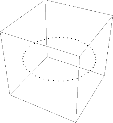
Graphics3D[Point[weeks]]

---

Update

Now that I have 10.2, here are the WhenEvent[] equivalents of the two code snippets given above:

G = 4 Pi^2 // N;
Reap[NDSolve[{r''[t] == -G r[t]/Norm[r[t]]^3, WhenEvent[t == 1, Sow[r[t]]],
              r[0] == {1, 0, 0}, r'[0] == {0, 2 Pi, 0}}, {}, (*empty!*)
             {t, 1}, Method -> "ExplicitRungeKutta", MaxStepSize -> 1/365]][[-1, 1, 1]]

weeks = Reap[NDSolve[{r''[t] == -G r[t]/Norm[r[t]]^3, 
                      WhenEvent[Mod[t, 7./365] == 0, Sow[r[t]]], 
                      r[0] == {1, 0, 0}, r'[0] == {0, 2 Pi, 0}}, {}, {t, 1},
                     Method -> "ExplicitRungeKutta", MaxStepSize -> 1/365]][[-1, 1]]

For some reason, though, the second snippet gives one less point than the version using "EventLocator".

Answer 4

One very pedestrian way could be to divide your total integration interval into smaller sub-intervals and then integrate over these smaller intervals, one at a time. The values of the variables (to be integrated) at the end of one of the sub-intervals are to be taken as the initial values for integration over the next sub-interval and so on.

Of course, the solution/product of NDSolve over a certain sub-interval is to overwritten by that got from integrating over the next sub-interval. So, instead of Mathematica having to store the solution over the entire integration interval, now it has to store over only one of the sub-intervals.

Here is an example with a simple harmonic oscillator differential equation

eqnArray1  = {rd'[t] == -r[t],      

rd[t] == r'[t] } ;       (*differential eqns.*)

eqnArray2  = { r[0] == -2 , rd[0] == 0} ;         (*inital conditions*)

eqnArray3  = {r, rd}  ;        (*variables to be integrated*)

tInitial = 0 ;          (*initial time*)

end = 100;          (*final time (overall)*)

nIntervals = 10 ;       (*number of sub-intervals*)
DT = (end -  tInitial)/nIntervals ;     (*size of each subinterval*)

Do[                     
sol = NDSolve[ Join[eqnArray1, eqnArray2],   eqnArray3, {t, tInitial, tInitial + DT}] ;
(*'sol' is the solution over only one such sub-interval, and not the \
entire interval from tInitial --> end *)

Do[
 eqnArray2[[i]] = ( ((eqnArray3[[i]]  )[
    tInitial + DT]) == ((eqnArray3[[i]]  ) /. 
     sol[[1]])[tInitial + DT])   ;
, {i, 1, Length[eqnArray3]}] ;
(*This Do loop sets the initial condition for the next sub-interval \
to be equal to the 
values of the variables at the end of the previous sub-interval*)

tInitial = tInitial + DT ;  
(*initial time of the next sub-interval is DT added to \
the initial time of the previous sub-interval*)

, {ii, 1,    
nIntervals}]  ;       (*this Do loop goes over every sub-interval \
until we reach 'end'*)

(r /. sol[[1]])[100]
(rd /. sol[[1]])[100]
(*Display the final solution*)