Gravitation simulation and interaction of N (1000) massive objects

Question

Is there an implementaion of the Barnes-Hut algorithm running with Mathematica? Thanks a lot

Answer 1

And I was somewhat lying in wait for this kind of question...

In I have been working on Barnes-Hut-like code for the so-called tangent-point energies in the last couple of years. This is a family of repulsive energies of curves and surface (see Yu, Schumacher, Crane - Repulsive Curves) and Yu, Schumacher, Crane - Repulsive Surfaces).

For a specific choice of parameters, this code allows us to also compute the forces of the Coulomb energy. Flip the signs and you get gravitation!

I would like to point out that I developed my code for a slightly different task. It is by far not optimal for OP's application -- but it does better than any naive all-pairs implementation.

For example, I do not use a regular octree, but a bounding value hierarchy. For (almost uniform) point clouds, the latter is more complicated to build than an octree. But it solves several issues that arise when the points are distributed on low-dimensional submanifolds of $\mathbb{R}^3$. Moreover, my code builds a couple of other things that are necessary for submanifolds that are trivial for point clouds. (E.g., checking self-intersections, keeping track of the tangent planes, assembling derivatives..)

In order to use the code below, you will have to follow several steps:

1. Go to github, create an account there.

2. Use git clone --recurse-submodules to clone the repository at https://github.com/HenrikSchumacher/Repulsor to a directory of choice on your local hard drive. Make sure to use git clone --recurse-submodules; this guarantees that some other required packages are also pulled into the correct subdirectories.

3. Open Mathematica. Input the path to the cloned repository into the variable $RepulsorIncludeDirectory in the code snippet below.

4. If you run this on macos, you can probably skip this step. Just make so to have the most recent version of XCode and the Command Line Tools installed. For other operating systems you will have to edit also the other compilation options. This should be fairly straight-forward. (But for the lack of a test system, I cannot do that for you.) Note that you need to link a BLAS and a LAPACK implementation. OpenBLAS should do. (On macos the BLAS and LAPACK routines from the Accelerate framework are used.)

5. Then run the snippet below. This will create a LibraryFunction. This takes quite some time (a minute or so).

The code:

(*You have to set this to the path that contains the file Repulsor.hpp.*)
$RepulsorIncludeDirectory = FileNameJoin[{$HomeDirectory,"github","Repulsor"}];

Needs["CCompilerDriver`"];
Quiet[LibraryFunctionUnload[cCoulomb]];
ClearAll[cCoulomb];
cCoulomb = Module[{lib,code,filename,name,time},
    name = "cCoulomb";
    filename = name;
    
    code = StringJoin["
#include \"WolframLibrary.h\"

#define LAPACK_DISABLE_NAN_CHECK
#define ACCELERATE_NEW_LAPACK
#include <Accelerate/Accelerate.h>
#include \"Repulsor.hpp\"

using Real = mreal;
using Int  = int;
using LInt = mint;

constexpr Int DomDim = 0;
constexpr Int AmbDim = 3;

using Mesh_T   = Repulsor::SimplicialMesh<DomDim,AmbDim,Real,Int,LInt,Real,Real>;

EXTERN_C DLLEXPORT int "<>name<>"(WolframLibraryData libData, mint Argc, MArgument *Args, MArgument Res)
{
    MTensor coords     = MArgument_getMTensor(Args[0]); 
    MTensor charges    = MArgument_getMTensor(Args[1]); 
    MTensor forces     = MArgument_getMTensor(Args[2]); 
    mreal alpha        = MArgument_getReal(Args[3]); 
    mreal theta        = MArgument_getReal(Args[4]); 
    mint  thread_count = MArgument_getInteger(Args[5]); 
    
    const Int n = static_cast<Int>(libData->MTensor_getDimensions(coords)[0]);

    Tensors::Tensor1<Int,Int> simplices = Tensors::iota<Int>(n);    

    Mesh_T M ( 
        libData->MTensor_getRealData(coords),  n, false,
        simplices.data(),                      n, false, 
        libData->MTensor_getRealData(charges), 
        thread_count 
    );
    
    M.cluster_tree_settings.split_threshold                      = 1;
    M.cluster_tree_settings.thread_count                         = thread_count;
    M.block_cluster_tree_settings.far_field_separation_parameter = theta;

    Repulsor::TangentPointEnergy<Mesh_T> E ( 0, alpha );    

    const mreal energy = 0.5 * E.Differential(M, libData->MTensor_getRealData(forces));
    
    Tensors::scale_buffer( 0.5, libData->MTensor_getRealData(forces), n * AmbDim );

    libData->MTensor_disown(forces);

    MArgument_setReal(Res, energy);
    
    return LIBRARY_NO_ERROR;
}"];

    Print["Compiling "<>name<>"..."];
    time= AbsoluteTiming[
        lib=CreateLibrary[code,filename,
            "Language"->"C++",
            "TargetDirectory"-> $TemporaryDirectory,
            "ShellOutputFunction"->Print,
            "CompileOptions" -> {
                " -Wall"
                ,"-Wextra"
                ,"-Wno-unused-parameter"
                ,"-gline-tables-only"
                ,"-gcolumn-info"
                ,"-mmacosx-version-min="<>StringSplit[Import["!sw_vers &2>1","Text"]][[4]]
                ,"-std=c++20"
                ,"-fno-math-errno"
                ,Switch[$SystemID
                    ,"MacOSX-ARM64","-mcpu=apple-m1 -mtune=native"
                    ,"MacOSX-x86-64","-march=native -mtune=native"
                    ,_,""
                ]
                ,"-Ofast","-flto","-pthread","-framework Accelerate"
                }
            ,"IncludeDirectories" -> {$RepulsorIncludeDirectory}
        ];
    ][[1]];
    
    Print["Compiling "<>name<>" done. Time elapsed = "<>ToString[time]<>"s."];
    
    LibraryFunctionLoad[lib,name,
        {
            {Real,2,"Constant"},  (* point coordinates as n x 3 matrix *)
            {Real,1,"Constant"},  (* point charges as n vector *)
            {Real,2,"Shared"},    (* forces for each point as n x 3 matrix (Caution, pass by reference!)*)
            Real,                 (* exponent of Coulomb-like potential; classical Coulomb potential has alpha = 1*)
            Real,                 (* separation parameter \[Theta]*)
            Integer               (* number of threads to use (Don't use more than the actual number of cores!)*)
        },
        Real                      (* return value: total Coulomb potential of point cloud. *)
    ]
];

If the compilation did not throw any errors, then you are ready to go!

Here a simple example: 5000 points uniformly distributed in a ball of radius 100 with random charges.

X = RandomPoint[Ball[{0, 0, 0}, 100], 5000];
{n, d} = Dimensions[X];

charges = RandomReal[{1., 2.}, n];

(*We have to preallocate this array so that the LibraryFunction cCoulomb can write to it.*)
forcesBH = ConstantArray[0., {n, d}];

(*The separation parameter for the so-called _mulitpole acceptance criterion_.*)
(* \[Theta] == 0. means that all point pairs are executed to obtain the exact net energy and the exact forces. *)
(* The larger \[Theta] is, the faster the force computation will be -- but also the greater the errors will get!*)
\[Theta] = 0.25;

(*Exponent for exponent for the Coulomb-like potential. \[Alpha] = is the classical Coulomb potential.*)
\[Alpha] = 1.;

threadCount = 
  "ParallelThreadNumber" /. ("ParallelOptions" /. SystemOptions["ParallelOptions"]);

timeBH = AbsoluteTiming[
    (*Beware, 
    forcesBH is overwriten as it is passed to energyBH _by reference_.*)
    (*This is quite untypical for Mathematica code.*)
    energyBH = 
      cCoulomb[X, charges, forcesBH, \[Alpha], \[Theta], 
       threadCount];
    ][[1]];

"Barnes-Hut computation time" -> timeBH

On my 8-core M1 Max processor, this takes about 0.02 seconds.

Let's see how long a single-threaded, pure top-level-Mathematica implementation with Do loops would take:

energyTrue = 0.;
forcesTrue = ConstantArray[0., {n, d}];
Dynamic[Row[{i, "/", n}]]

timeTrue = AbsoluteTiming[
    Do[
      Block[{x, c},
       x = X[[i]];
       c = charges[[i]];
       Do[
        Block[{v, cc, r2, r, force},
         v = X[[j]] - x;
         r2 = v . v;
         r = Sqrt[r2];
         
         cc = c charges[[j]];
         
         force = cc v /(r r2);
         forcesTrue[[i]] += force;
         forcesTrue[[j]] -= force;
         
         energyTrue += cc/r;
         ]
        , {j, i + 1, n}]
       ]
      , {i, 1, n}];
    ][[1]];
"Full computation time" -> timeTrue
"Speed-up" -> timeTrue/timeBH

"Full computation time" -> 67.7153

"Speed-up" -> 2501.49

Note that a major portion of the speed-up can simply be traced back to the fact that cCoulomb is implemented in C++ and that most of its parts are parallelized.

What about the accuracy?

forceErrors = (Norm /@ (forcesBH - forcesTrue));
forceMagnitudes = (Norm /@ forcesTrue);
forceRelErrors = forceErrors/forceMagnitudes;

"Energy relative error" -> Abs[(energyBH - energyTrue)/energyTrue]
"Forces relative error (max)" -> Max[forceErrors/forceMagnitudes]
"Forces relative error (mean)" -> Mean[forceErrors/forceMagnitudes]

"Energy relative error" -> 0.000594074

"Forces relative error (max)" -> 0.253584

"Forces relative error (mean)" -> 0.0346127

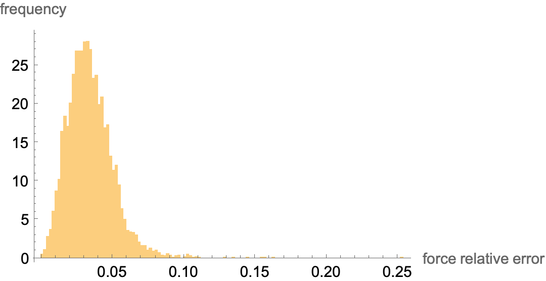
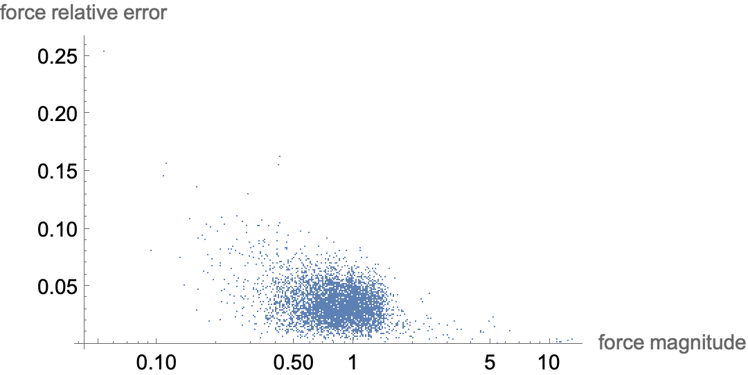
There are some few severe outliers, but they typically appear only for points whose force magnitude is rather smallish. On average, this approximation is quite okay:

ListPlot[
 Transpose[{forceMagnitudes, forceRelErrors}],
 PlotRange -> All,
 ScalingFunctions -> {"Log", "Linear"},
 AxesLabel -> {"force magnitude", "force relative error"}
 ]

Histogram[forceRelErrors,
 "Wand", "PDF", PlotRange -> All,
 AxesLabel -> {"force relative error", "frequency"}
 ]

On my machine, cCoulomb manages to handle about 467000 points per second. And its runtine scales roughly linearly with the number of points. This seems to be okay, but I have seen implementations that claim to handle several times as many points per second on similar hardware (albeit with a substantially larger separation parameter) (see e.g., rakau).

So if you want to do a large-scale simulation, you should rather look for these implementation (which will be very likely in C or C++) and link them with LibraryLink.