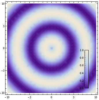
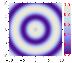
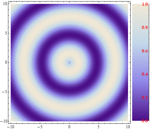
49
$\begingroup$

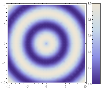
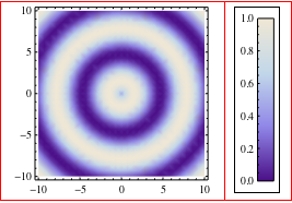
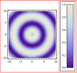
I would like to add a colour bar to a plot. I tried to use GraphicsRow for this. In a GraphicsRow, each item is given the same space, resulting in this:

Clear[colorbar]
colorbar[colorFunction_: Automatic, divs_: 25] := 
 DensityPlot[y, {x, 0, .1}, {y, 0, 1}, AspectRatio -> Automatic, 
  PlotRangePadding -> 0, PlotPoints -> {2, divs}, MaxRecursion -> 0, 
  FrameTicks -> {None, Automatic, None, None}, 
  ColorFunction -> colorFunction]

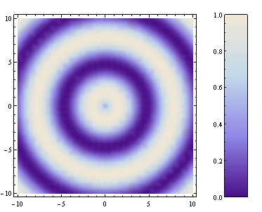
GraphicsRow[{DensityPlot[Sin[Norm[{x, y}]], {x, -10, 10}, {y, -10, 10}],
             colorbar[]}]
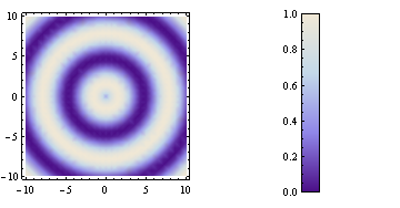
Mathematica graphics

The colour bar has too much space around it. How can I specify the amount of space GraphicsRow should give a particular item?

Alternatively, what is a better way to include the colour bar?


Answer summary

After experimenting with this for a while, it seems that the situation is the following (simplified):

  • Grid and friends (Row, Column) will size the grid cells to fit each item individually (cells resized to fit items).

  • GraphicsGrid will first set up a grid with fixed cell sizes, then fit each item into the cells (items resized to fit cells).

GraphicsGrid-like solutions are more convenient when the whole graphic need to be sized to a specification.

István's answer hacks GraphcisRow by setting a negative spacing and thus pushing the elements closer together. It's the most convenient for this situation, but it doesn't generalize for many cells.

R.M.'s solution suggests using Grid instead. This generalizes well, but requires pre-sizing all items individually, and no resizing is possible after (e.g. just before import).

Since GraphicsGrid is implemented in terms of Inset, the most general easily resizable solution would be implementing a GraphicsGrid-like construct where cell size ratios can be specified. kguler's last answer illustrates this best.

Several other solutions used Inset directly as well. A problem with resizing these solutions can be that the aspect ratio of elements is size-dependent (due to the absolute sizes used in ImagePadding), so how they fit into a fixed aspect ratio Inset will depend on the scale. Note for example the difference in scaling behaviour between István's solution and kguler's solution at small sizes: in kguler's solution (using a cell aspect ratio matching that of the colour bar) the colourbar suddenly get shrunk compared to the main plot at small sizes, but the tick marks will never overlap with the other plot. in István's solution (which uses overlapping square cells) the colour bar never gets overshrunk, but the tick marks will overlap the main plot.

Update: Version 9 has built-in support for plot legends, including colour bars. Legended is used to append a legend to a graphics object.

$\endgroup$
7
  • $\begingroup$ What is wrong with Grid rather than GraphicsRow/ GraphicsGrid? The sizings are not fixed to be equal with Grid. $\endgroup$
    – Verbeia
    Commented Feb 20, 2012 at 20:12
  • $\begingroup$ @Verbeia Now I see that Grid is the most workable solution. The inconvenience is that it's not resizable. I need to specify the size of the grid elements instead. I am making all my figures to size, and I don't resize the final result in LaTeX because I want the font sizes to be consistent. Resizing in Mathematica does not alter font sizes, but resizing an exporting PDF does. That said, I am going with Grid, as R.M. suggested. I don't think there is any other usable option. (I actually manged to tweak the cell sizes in GraphicsRow, but it introduced other problems.) $\endgroup$
    – Szabolcs
    Commented Feb 20, 2012 at 20:32
  • $\begingroup$ ItemSize option to Grid? Let me see if I can come up with an answer quickly before work beckons. $\endgroup$
    – Verbeia
    Commented Feb 20, 2012 at 20:41
  • $\begingroup$ @Verbeia When I use Grid, ItemSize is not even necessary because it the cells will auto-size to the content. $\endgroup$
    – Szabolcs
    Commented Feb 20, 2012 at 21:16
  • $\begingroup$ It's useful if your original ImageSize on the colorbar is not conformable to the other plot (which it isn't by default on my screen). Yes, you can use R.M.'s answer using Show, but in case there are situations where you don't want to use Show, this works. See the edit to my answer. $\endgroup$
    – Verbeia
    Commented Feb 20, 2012 at 21:22

8 Answers 8

28
$\begingroup$

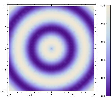
One way of doing it is to use Row instead of GraphicsRow and setting an explicit ImageSize. The solution also scales for different sizes. Setting the same ImagePadding on both plots will ensure that they are nicely aligned. For example:

With[{size = 300}, 
 Row[Show[#, ImageSize -> {Automatic, size}, 
     ImagePadding -> 20] & /@ {DensityPlot[
     Sin[Norm[{x, y}]], {x, -10, 10}, {y, -10, 10}], colorbar[]}]]

Mathematica graphics


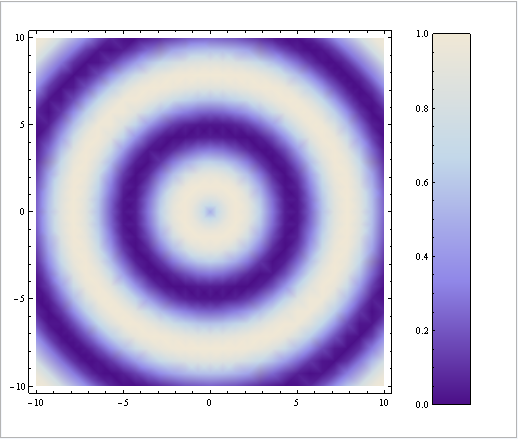
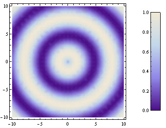
The above plot still has excess spacing between the graphic and the color bar. The reason for this is because of the uniform padding of 20. So this translates to 20 for the right side of the first + 20 for the left side of the second which means a 40 total between the two. Using the {{left, right}, {bottom, top}} spacing specification for ImagePadding works very well in aligning color bars to a plot. For this case, modify the above code to: ImagePadding -> {{20, 0}, {20, 5}}, which results in

enter image description here

You can now set a separate right padding if you need to leave some more space between the two.

$\endgroup$
12
$\begingroup$

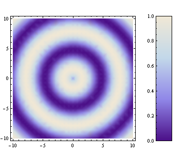
You can overlap GraphicsRow items by specifying negative spacings. This omits whitespace to the right (as in kguler's answer):

size = 360;

colorbar[colorFunction_: Automatic, divs_: 25] := 
 DensityPlot[y, {x, 0, .1}, {y, 0, 1}, AspectRatio -> Automatic, 
  PlotRangePadding -> 0, PlotPoints -> {2, divs}, MaxRecursion -> 0, 
  FrameTicks -> {None, Automatic, None, None}, 
  ColorFunction -> colorFunction, ImageSize -> {size/5, size}]

GraphicsRow[
 Show[#, ImagePadding -> 20] & /@ {DensityPlot[
    Sin[Norm[{x, y}]], {x, -10, 10}, {y, -10, 10}, ImageSize -> size],
    colorbar[]}, Alignment -> Right, ImageSize -> size, Frame -> None,
  Spacings -> {-3 size/4, Automatic}]

Mathematica graphics

Updated with appropriate size specifications.

$\endgroup$
1
  • $\begingroup$ I chose this because it has the best scaling behaviour and is simple to implement. $\endgroup$
    – Szabolcs
    Commented Feb 21, 2012 at 10:21
10
$\begingroup$

Using GraphicsRow options:

- Alignment option

  GraphicsRow[{DensityPlot[
  Sin[Norm[{x, y}]], {x, -10, 10}, {y, -10, 10}], colorbar[]}, 
  Alignment -> Left]

gives

legend in graphicsRow

- Spacings with negative values:

 GraphicsRow[{DensityPlot[
 Sin[Norm[{x, y}]], {x, -10, 10}, {y, -10, 10}], colorbar[]}, 
 Spacings -> Scaled[-.4]]

or

 GraphicsRow[{DensityPlot[
 Sin[Norm[{x, y}]], {x, -10, 10}, {y, -10, 10}], colorbar[]}, 
 Spacings -> -100]

Both give less white space on the right.

Replacing position and size options of Inset

Inspecting the InputForm of the output from GraphicsRow, we see that it is a collection of Inset objects, one for each graphics object in the argument list. So the positions and sizes of the graphics objects can be controlled by options to Inset. These are

Inset[obj,pos,opos]

aligns the inset so that position opos in the object lies at position pos in the enclosing graphic.

Inset[obj,pos,opos,size]

specifies the size of the inset in the coordinate system of the enclosing graphic.

This suggests a hack (specific to the example and wrapped with Panel to show the relative sizes)

 a = 420; b = 120; 
 Panel@GraphicsRow[{DensityPlot[
 Sin[Norm[{x, y}]], {x, -10, 10}, {y, -10, 10}], 
 Graphics[colorbar[]]}, ImageSize -> 500] /. Inset[gr_, 
   {576., pos2_}, ImageScaled[{0.5, 0.5}], {sz1_, sz2_}] :> 
Inset[gr, 
   {a, pos2}, ImageScaled[{0.5, 0.5}], {b , sz2}]

with output

inset legend

DIY GraphicsRow: Using Graphics and Inset:

Use Graphics and Inset to replicate what GraphicsRow does, and control the options for Inset directly:

 Graphics[{ {Inset[
 DensityPlot[Sin[Norm[{x, y}]], {x, -10, 10}, {y, -10, 10}], 
    {192, -189.}, ImageScaled[{0.5, 0.5}], {360, 360.}], 
  Inset[Graphics[colorbar[]], 
    {420., -189.}, ImageScaled[{0.5, 0.5}], {120., 360.}]}}, 
ContentSelectable -> True, ImageSize -> 500,
PlotRangePadding -> {6, 5}]

which produces the same output.

$\endgroup$
1
  • $\begingroup$ I found this myself, but unfortunately there's still a lot of whitespace on the right, which causes trouble when I export this to include in a document. $\endgroup$
    – Szabolcs
    Commented Feb 20, 2012 at 18:28
9
$\begingroup$

Further to R.M.'s answer, you can use some combination of ImageSize on the graphic elements and ItemSize for the Grid elements themselves to finesse spacing. I've added the possibility to include other options to the colorbar function, such as ImageSize, though if you use them you need to set the other two arguments explicitly. This is an alternative to Show with additional options.

colorbar[colorFunction_: Automatic, divs_: 25, 
  opts : OptionsPattern[]] := 
 DensityPlot[y, {x, 0, .1}, {y, 0, 1}, 
  Evaluate[Sequence @@ FilterRules[{opts}, Options[DensityPlot]]], 
  AspectRatio -> Automatic, PlotRangePadding -> 0, 
  PlotPoints -> {2, divs}, MaxRecursion -> 0, 
  FrameTicks -> {None, Automatic, None, None}, 
  ColorFunction -> colorFunction]

Framed to show the difference between ItemSize and ImageSize. Note that the former is in character widths and the latter is in pixels.

Grid[{{DensityPlot[Sin[Norm[{x, y}]], {x, -10, 10}, {y, -10, 10}], 
   Framed@colorbar[Automatic, 30, ImageSize -> 32]}}, 
 ItemSize -> {{15, 4}}, Frame -> All, FrameStyle -> Red]

enter image description here

This alternative might be useful if, like here, the default sizes don't quite work together, and for whatever reason you don't want to use Show.

enter image description here

$\endgroup$
1
  • $\begingroup$ This is quite nice looking $\endgroup$
    – Szabolcs
    Commented Feb 20, 2012 at 21:21
9
$\begingroup$

This is a little late, but I had actually fought the same problem a couple of days ago, and only now saw that this was a question. I'm putting it here as another solution:

Clear[colorbar,defaultSize]
defaultSize=360;

colorbar[colorFunction_: Automatic, divs_: 25] := 
 DensityPlot[y, {x, 0, .1}, {y, 0, 1}, PlotRangePadding -> 0, 
  PlotPoints -> {2, divs}, AspectRatio -> Full, 
  ImageSize -> {defaultSize/10, defaultSize}, MaxRecursion -> 0, 
  FrameTicks -> {None, Automatic, None, None}, 
  ColorFunction -> colorFunction]

GraphicsRow[{DensityPlot[
   Sin[Norm[{x, y}]], {x, -10, 10}, {y, -10, 10}, ImageSize -> defaultSize], 
  colorbar[]}, Alignment -> {Left, Center}, Spacings -> 20, 
 ImageSize -> {Automatic, defaultSize}]

The difference between the original question and this is the following:

  1. AspectRatio->Full which according to the docs: "specifies that a graphic should be stretched so as to fill out its enclosing region in a Grid or related construct."

  2. Explicit ImageSize, especially in the GraphicsRow to specify Automatic in the horizontal direction, but our default size in the vertical.

  3. Alignment->{Left,Center}

  4. Spacings played around with until a 'nice' value was found.

Hope this helps someone. FWIW, I have no idea why the above works, maybe someone better versed in inner MMA speak can answer that.

DensityPlot

$\endgroup$
3
  • $\begingroup$ Interesting solution, I didn't know about AspectRatio -> Full. Thanks for sharing! $\endgroup$
    – Szabolcs
    Commented Mar 1, 2012 at 21:21
  • $\begingroup$ @Szabolcs you're welcome. I had more or less the exact same problem, and it took me a full day to figure out the right combo of settings. It's voodoo. $\endgroup$
    – tkott
    Commented Mar 1, 2012 at 21:22
  • $\begingroup$ I used the answer I accepted in conjunction with this. What a hack to use image processing just to get some margins right! $\endgroup$
    – Szabolcs
    Commented Mar 1, 2012 at 21:27
7
$\begingroup$

This seems to give good flexibility:

Show[DensityPlot[Sin[Norm[{x, y}]], {x, -10, 10}, {y, -10, 10}], 
 Graphics@Inset[colorbar[], {15, 0}], 
 ImagePadding -> {{20, 100}, {20, 20}}, PlotRangeClipping -> False]

enter image description here

EDIT: You can also use relative coordinates:

Graphics@Inset[colorbar[], ImageScaled[{0.9, 0.5}]]

The advantage of this method is that you can easily configure/tweak it to be almost anything you want, and also add multiple Graphics:

Show[DensityPlot[Sin[Norm[{x, y}]], {x, -10, 10}, {y, -10, 10}], 
 Graphics@Inset[colorbar[], ImageScaled[{1, 0.3}], {0.5, 0.5}, 
   ImageScaled[{0.1, 0.4}]], ImagePadding -> {{20, 20}, {20, 20}}]

enter image description here

$\endgroup$
3
  • $\begingroup$ The disadvantage here is that the positioning of the colour bar depends on the plot coordinates on the main graphic --- something to avoid if possible. $\endgroup$
    – Szabolcs
    Commented Feb 20, 2012 at 18:35
  • $\begingroup$ @Szabolcs I edited it with an example independent of the plot coordinates $\endgroup$
    – P. Fonseca
    Commented Feb 20, 2012 at 18:50
  • $\begingroup$ Placing the colour bar inside the plot is not acceptable for my use case. The entire plot region contains important information that must not be covered. Thank you for showing be ImageScaled, it will prove very useful! $\endgroup$
    – Szabolcs
    Commented Feb 20, 2012 at 19:11
2
$\begingroup$

Mathematica versions 11 and 12 behave differently with regard to GraphicsRow/GraphicsGrid.

For GraphicsRow, there is no change required when using the negative spacing hack identified as István's answer in the Question's Answer Summary.

For GraphicsGrid, the negative spacing hack which worked in version 11 does not immediately in version 12. Calling AspectRatio as outlined in a related post allows keeping previously chosen spacing(s) as is. Besides, both versions 11 and 12 result in whitespace at the top. If neither using Frame nor Dividers, that can be removed with ImageCrop, see e.g. there.

$\endgroup$
1
$\begingroup$

This is the best scaling behavior for this specific problem that I could come up with:

Clear[colorbar]
colorbar[colorFunction_: Automatic, divs_: 25] := 
 DensityPlot[y, {x, 0, .1}, {y, 0, 1},
   PlotPoints -> {2, divs}, MaxRecursion -> 0,
   AspectRatio -> 7, PlotRangePadding -> 0,  
   Frame -> False, Axes -> {False, True}, 
   TicksStyle -> Directive[Bold, Red], AxesOrigin -> {0.1}, 
   ColorFunction -> colorFunction
 ]

Graphics[{
  First @ DensityPlot[Sin[Norm[{x, y}]], {x, -10, 10}, {y, -10, 10}],
  Inset[
    colorbar[],
    Scaled[{1, 1/2}],
    ImageScaled[{-0.1, 1/2}],
    Scaled[{1/7, 1}]
  ]
 },
 Frame -> True,
 ImagePadding -> {{Automatic, Automatic}, {Automatic, 5}}
]

Mathematica graphics

Mathematica graphics

$\endgroup$
1
  • 1
    $\begingroup$ Nice trick putting the ticks inside. Unfortunately I can't do this. But I learned about the possibility of FrameTicks -> {None, None, None, All} now. Thanks! (That All was not so obvious to me.) $\endgroup$
    – Szabolcs
    Commented Feb 21, 2012 at 12:59

Your Answer

By clicking “Post Your Answer”, you agree to our terms of service and acknowledge you have read our privacy policy.

Not the answer you're looking for? Browse other questions tagged or ask your own question.