Here's a method that is a generalization of this one and should work for arbitrary $n$ and $m$. It is very efficient, as long as you don't want to do a graphics plot as below.
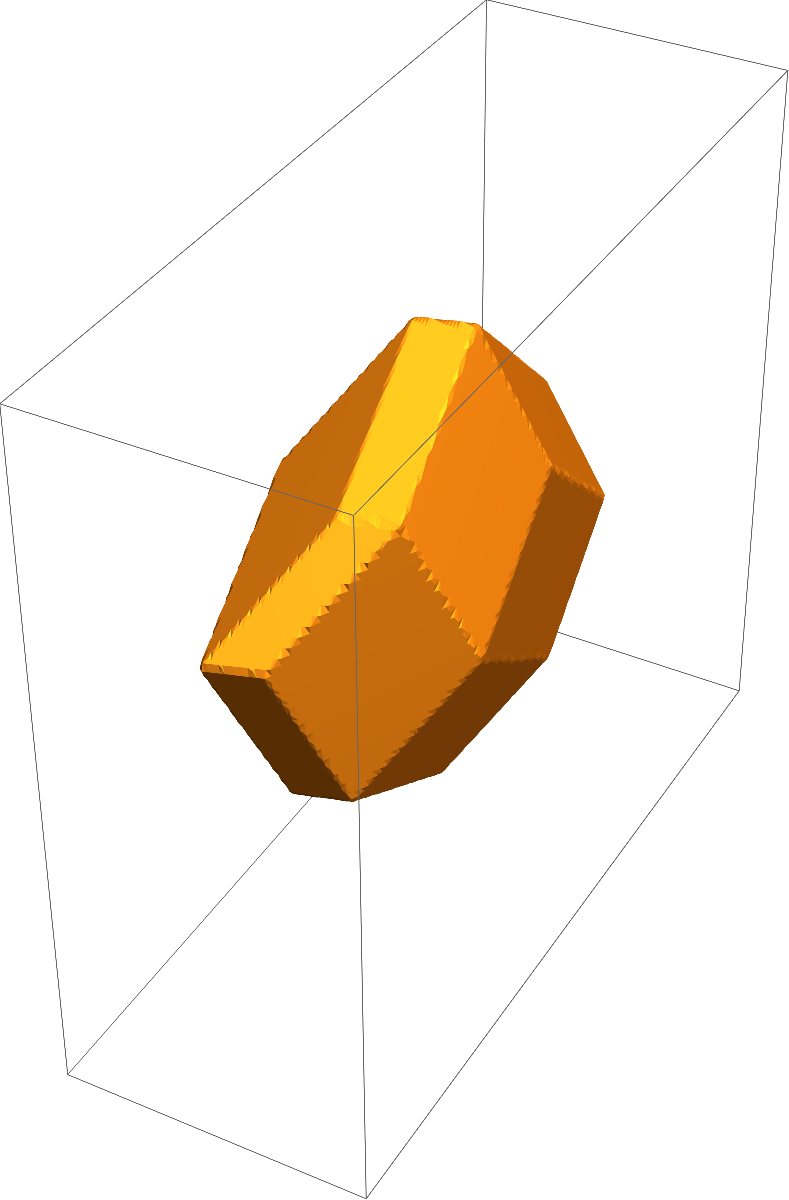
Let's do a random example where $m=3$ so we can visualize the polytope in 3D:
n = 5;
m = 3;
M = RandomVariate[NormalDistribution[], {m, n}]
(*    {{-0.304994, -0.392532, 0.823638, -0.201907, 0.108934},
       {-0.100295, -0.66419, -2.50501, -0.483007, -0.982172},
       {0.00520204, -0.601936, 1.99376, 1.07407, -0.579136}}    *)
To calculate the facet normals, we take all length-$(m-1)$ tuples of columns of $M$, and for each such tuple calculate the vector that is perpendicular to all of them (via NullSpace):
W = Join @@ NullSpace /@ Subsets[Transpose[M], {m - 1}]
(*    {{0.250025, -0.727159, 0.639318},
       {-0.176108, 0.576911, 0.797596},
       {-0.287587, 0.89256, 0.34732},
       {0.174337, -0.485727, 0.856549},
       {-0.876301, 0.0887525, 0.473518},
       {-0.878533, 0.475208, 0.0485508},
       {-0.355215, -0.50372, 0.787457},
       {0.739474, 0.55098, 0.386781},
       {-0.968459, -0.197213, 0.152295},
       {0.982782, 0.0000529691, 0.184769}}    *)
In this case, there are $\binom{n}{m-1}=\binom{5}{2}=10$ such facet normals. For each facet we use the linear programming trick of your previous question to get the minimum and maximum values of the scalar product with this facet normal, to find the boundaries of the polytope:
w = {#.LinearProgramming[#, -IdentityMatrix[n, SparseArray], ConstantArray[-1,n]],
     #.LinearProgramming[-#, -IdentityMatrix[n, SparseArray], ConstantArray[-1,n]]} & /@ (W.M)
(*    {{0., 4.66071}, {-1.84188, 0.613583}, {-3.57839, 0.},
       {-0.261406, 4.1875}, {-0.456861, 0.903485}, {-2.40775, 0.220539},
       {0., 3.86301}, {-1.85243, 0.}, {0., 1.18978},
       {-0.795815, 1.17771}}    *)
We can now assemble the inequalities that describe the polytope's facets, using the facet normals W and the associated scalar-product ranges w:
Y = Array[y, m];
F = And @@ MapThread[#2[[1]] <= #1.Y <= #2[[2]] &, {W, w}]
(*    0. <= 0.250025 y[1] - 0.727159 y[2] + 0.639318 y[3] <= 4.66071 &&
      -1.84188 <= -0.176108 y[1] + 0.576911 y[2] + 0.797596 y[3] <= 0.613583 &&
      -3.57839 <= -0.287587 y[1] + 0.89256 y[2] + 0.34732 y[3] <= 0. &&
      -0.261406 <= 0.174337 y[1] - 0.485727 y[2] + 0.856549 y[3] <= 4.1875 &&
      -0.456861 <= -0.876301 y[1] + 0.0887525 y[2] + 0.473518 y[3] <= 0.903485 &&
      -2.40775 <= -0.878533 y[1] + 0.475208 y[2] + 0.0485508 y[3] <= 0.220539 &&
      0. <= -0.355215 y[1] - 0.50372 y[2] + 0.787457 y[3] <= 3.86301 &&
      -1.85243 <= 0.739474 y[1] + 0.55098 y[2] + 0.386781 y[3] <= 0. &&
      0. <= -0.968459 y[1] - 0.197213 y[2] + 0.152295 y[3] <= 1.18978 &&
      -0.795815 <= 0.982782 y[1] + 0.0000529691 y[2] + 0.184769 y[3] <= 1.17771    *)
To show the polytope:
J = ImplicitRegion[F, Evaluate@Y];
RegionPlot3D[J, PlotPoints -> 100]

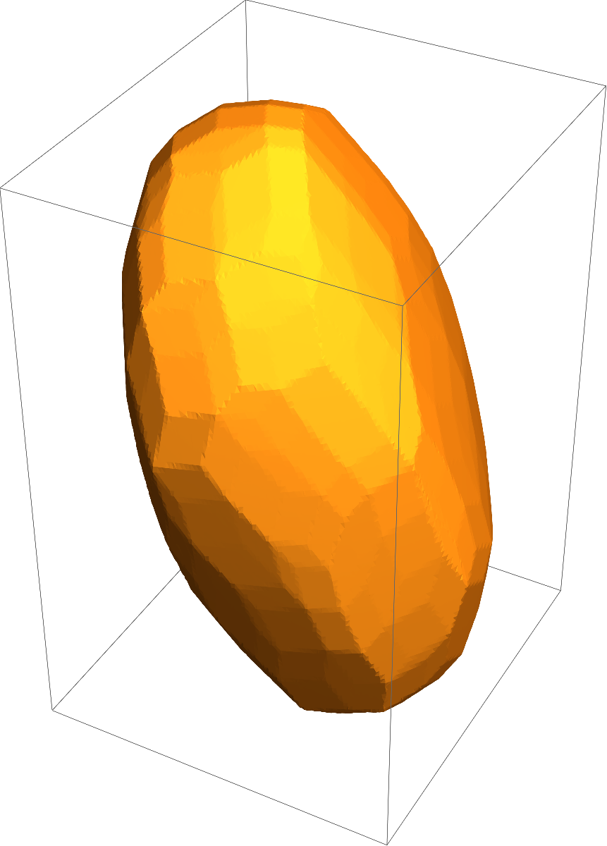
To show off, let's do this for n=20 and m=3: we get $\binom{20}{2}=190$ facet normals, 380 inequalities, and an almost ellipsoidal polytope:


mandn? Ismgreater or smaller thann. And what do you want to do with the result? $\endgroup$Y, you simply have to test whetherPseudoInverse[M].Ylies in the unit cube. Since the pseudoinversePseudoInverse[M]may look pretty complicated whenMis given symbolically, I suggest to do the computation ofPseudoInverse[M]numerically. $\endgroup$Yfor whichPseudoInverse[M].Ylies in the unit hypercube. How do you parametrize the faces of this convex polyhedron as inequalities? $\endgroup$Ydoes there exist any pseudoinversePsuch thatP.Ylies in the unit-hypercube. So you need to search over the space of pseudo-inverses. $\endgroup$P = Tuples[{0, 1}, n].Transpose[M]and then try to find the convex hull of these points withConvexHullMesh[P]. But this seems like a terrible idea. $\endgroup$