7
$\begingroup$

I'm trying to model the solar system with NDSolve, basically a numerical n-body solution.

I model the initial positions of bodies from a data set thusly:

{"sun", 
 {-1.068000648301820*^9, -4.176802125684930*^8, 3.084467020687090*^7},
 {9.305300847631915, -1.283176670344807*10,-1.631528028381386*^-1}, 
 1.988544*^30, White}

Where the first triplet is the body's initial position with regard to the solar system's barycentre, the second triplet its initial velocity, and the fourth position number its mass.

The NDSolve, then evaluates the law of gravitation with respect to all tuples of masses in Cartesian component form.

This works fine for the major bodies. I'm currently getting roughly 3-4 accurate significant numbers after a setting the time of the model to 1 year.

My problem is with modelling the asteroid belt. Naturally, I can't model it as a single point particle. So I was wondering if there is a way to model it as a distribution with mass $3\times10^{21}$. I'm really only interested in finding a way to have the asteroid belt excert its gravitational influence on other bodies.

Here is a minimal working example, if I understand how to do it here, I can work out how to incorporate it in the actual model.

Supposing I started with a very simple model of one planet (sun+earth):

G = 6.6740831*10^-11;
{m1,m2} = {1.98855*^30, 5.97237*^24};
a = {x1''[
     t] == (G m2) (-x1[t] + 
        x2[t])/((-x1[t] + x2[t])^2 + (-y1[t] + y2[t])^2 + (-z1[t] + 
            z2[t])^2)^(3/2), 
   x2''[
     t] == (G m1) (-x2[t] + 
        x1[t])/((-x2[t] + x1[t])^2 + (-y1[t] + y2[t])^2 + (-z1[t] + 
            z2[t])^2)^(3/2), 
   y1''[
     t] == (G m2) (-y1[t] + 
        y2[t])/((-x1[t] + x2[t])^2 + (-y1[t] + y2[t])^2 + (-z1[t] + 
            z2[t])^2)^(3/2), 
   y2''[
     t] == (G m1) (-y2[t] + 
        y1[t])/((-x2[t] + x1[t])^2 + (-y1[t] + y2[t])^2 + (-z1[t] + 
            z2[t])^2)^(3/2), 
   z1''[
     t] == (G m2) (-z1[t] + 
        z2[t])/((-x1[t] + x2[t])^2 + (-y1[t] + y2[t])^2 + (-z1[t] + 
            z2[t])^2)^(3/2), 
   z2''[
     t] == (G m1) (-z2[t] + 
        z1[t])/((-x2[t] + x1[t])^2 + (-y1[t] + y2[t])^2 + (-z1[t] + 
            z2[t])^2)^(3/2)};
vel = {{Derivative[1][x1][0] == 0, 
    Derivative[1][x2][0] == 0}, {Derivative[1][y1][0] == -0.0894406, 
    Derivative[1][y2][0] == 29780}, {Derivative[1][z1][0] == 0, 
    Derivative[1][z2][0] == 0}};
pos = {{x1[0] == 0, x2[0] == 152100000000}, {y1[0] == 0, 
    y2[0] == 0}, {z1[0] == 0, z2[0] == 0}};
var = {x1, x2, y1, y2, z1, z2};
tmax = 3600*24*365.24;
s = NDSolve[Flatten[{a, vel, pos}], var, {t, 0, tmax}];
ParametricPlot3D[
Flatten[Thread[{{x1[t], y1[t], z1[t]}, {x2[t], y2[t], z2[t]}} /.s]],
{t, 0, tmax}, 
PlotRange -> {{-2*^11, 2*^11}, {-2*^11, 2*^11}, {-0.5*^11, 0.5*^11}}]

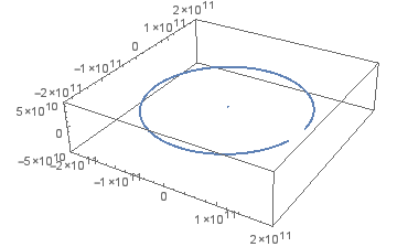
enter image description here

This doesn't make a complete orbit in one year, but obviously the accuracy here is low. Where a is the acceleration vectors ,vel the velocities, and pos the positions.

$\endgroup$
10
  • $\begingroup$ While it doesn't answer your mass question, you really should be in vector form here: X1[t_] = {x1[t], y1[t], z1[t]};X2[t_] = {x2[t], y2[t], z2[t]}; eqns = {X1''[t] == (g m2 (X2[t] - X1[t]))/Norm[(X2[t] - X1[t])]^3, X2''[t] == (g m1 (X1[t] - X2[t]))/Norm[(X2[t] - X1[t])]^3}; s = NDSolve[{eqns, vel, pos}, {X1[t], X2[t]}, {t, 0, tmax}]; $\endgroup$
    – SPPearce
    Commented Jul 19, 2016 at 14:47
  • $\begingroup$ You could also label the vectors with an index, e.g. X[1][t_] or X["sun"][t_] etc, and that lets you iterate over those. $\endgroup$
    – SPPearce
    Commented Jul 19, 2016 at 14:49
  • 4
    $\begingroup$ In a computation giving only 3-4 significant digits over a year, I strongly suspect the asteroid belt objects have no detectable effect on the major bodies of the solar system. $\endgroup$
    – m_goldberg
    Commented Jul 19, 2016 at 14:52
  • 2
    $\begingroup$ I would recommend working in something like N-body units. Keeping around all those factors of ten can be a problem, precision-wise, I think. $\endgroup$
    – march
    Commented Jul 19, 2016 at 15:22
  • 1
    $\begingroup$ Well, scaling quantities in a reasonable set of units is a good skill to have in any situation, really. You want as many of the parameters to be on the order of 1 as possible. $\endgroup$
    – march
    Commented Jul 19, 2016 at 16:30

1 Answer 1

6
$\begingroup$

Because the Asteroid belt's mass is negligible (only 4% of the Moon's mass), it is not very efficient to include it in your simulations. However, if you still want to include it in your simulations, I suggest two methods for approximation:

  • Only consider the most massive objects in the asteroid belt (i.e Ceres, Vesta, etc), which include more than 50 percent of the belt's total mass
  • Use the gravitational field of a thin torus to consider the effects of the Asteroid belt. you can use different approximation formulas for planets outside and inside the asteroid belt, which can be found here

UPDATE

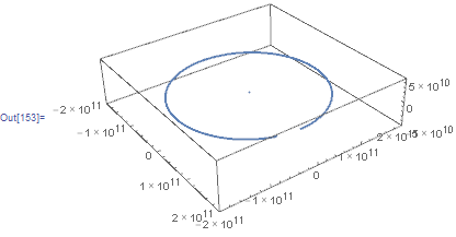
I've tried to use an approximation for the gravitational field of a torus-shaped asteroid belt for the Sun and Earth's orbit. If I have implemented the code correctly, then it shows how little can be the effect of the asteroid belt on the solar system. I have estimated the belt's Radius to be about 2.5 AU.

G = 6.6740831*10^-11;
AU =2.5*152100000000;
F[r_, R_] := (Block[{x = r/R}, (3.14159 x^2 + 
      3.5342917352885173` x^4 + 3.6815538909255383` x^6)/(2 Pi R^2)]);
{m1, m2, m3} = {1.98855*^30, 5.97237*^24, 3.*10^21};
a = {x1''[t] == (G m2) (-x1[t] + 
         x2[t])/((-x1[t] + x2[t])^2 + (-y1[t] + y2[t])^2 + (-z1[t] + 
             z2[t])^2)^(3/2) + 
     G m3 F[EuclideanDistance[{x1[t], y1[t], z1[t]}, {x3[t], y3[t], 
         z3[t]}], AU] ( 
       Normalize[{x1[t], y1[t], z1[t]} - {x3[t], y3[t], z3[t]}][[1]]),
   x2''[t] == (G m1) (-x2[t] + 
         x1[t])/((-x2[t] + x1[t])^2 + (-y1[t] + y2[t])^2 + (-z1[t] + 
             z2[t])^2)^(3/2) + 
     G m3 F[EuclideanDistance[{x2[t], y2[t], z2[t]}, {x3[t], y3[t], 
         z3[t]}], 
       AU] (Normalize[{x2[t], y2[t], z2[t]} - {x3[t], y3[t], 
           z3[t]}][[1]]),
   x3''[t] == -G m1 F[
       EuclideanDistance[{x1[t], y1[t], z1[t]}, {x3[t], y3[t], 
         z3[t]}], 
       AU] Normalize[{x1[t], y1[t], z1[t]} - {x3[t], y3[t], 
          z3[t]}][[1]] - 
     G m2 F[EuclideanDistance[{x2[t], y2[t], z2[t]}, {x3[t], y3[t], 
         z3[t]}], 
       AU] (Normalize[{x2[t], y2[t], z2[t]} - {x3[t], y3[t], 
           z3[t]}][[1]])
   , y1''[t] == (G m2) (-y1[t] + 
         y2[t])/((-x1[t] + x2[t])^2 + (-y1[t] + y2[t])^2 + (-z1[t] + 
             z2[t])^2)^(3/2) + 
     G m3 F[EuclideanDistance[{x1[t], y1[t], z1[t]}, {x3[t], y3[t], 
         z3[t]}], AU] ( 
       Normalize[{x1[t], y1[t], z1[t]} - {x3[t], y3[t], z3[t]}][[2]]),
    y2''[t] == (G m1) (-y2[t] + 
         y1[t])/((-x2[t] + x1[t])^2 + (-y1[t] + y2[t])^2 + (-z1[t] + 
             z2[t])^2)^(3/2) + 
     G m3 F[EuclideanDistance[{x2[t], y2[t], z2[t]}, {x3[t], y3[t], 
         z3[t]}], 
       AU] (Normalize[{x2[t], y2[t], z2[t]} - {x3[t], y3[t], 
           z3[t]}][[2]]), 
   y3''[t] == -G m1 F[
       EuclideanDistance[{x1[t], y1[t], z1[t]}, {x3[t], y3[t], 
         z3[t]}], 
       AU] Normalize[{x1[t], y1[t], z1[t]} - {x3[t], y3[t], 
          z3[t]}][[2]] - 
     G m2 F[EuclideanDistance[{x2[t], y2[t], z2[t]}, {x3[t], y3[t], 
         z3[t]}], AU] ( 
       Normalize[{x2[t], y2[t], z2[t]} - {x3[t], y3[t], z3[t]}][[2]]),
    z1''[t] == (G m2) (-z1[t] + 
         z2[
          t])/((-x1[t] + x2[t])^2 + (-y1[t] + y2[t])^2 + (-z1[t] + 
             z2[t])^2)^(3/2) + 
     G m3 F[EuclideanDistance[{x1[t], y1[t], z1[t]}, {x3[t], y3[t], 
         z3[t]}], AU] ( 
       Normalize[{x1[t], y1[t], z1[t]} - {x3[t], y3[t], z3[t]}][[3]]),
    z2''[t] == (G m1) (-z2[t] + 
         z1[t])/((-x2[t] + x1[t])^2 + (-y1[t] + y2[t])^2 + (-z1[t] + 
             z2[t])^2)^(3/2) + 
     G m3 F[EuclideanDistance[{x2[t], y2[t], z2[t]}, {x3[t], y3[t], 
         z3[t]}], 
       AU] (Normalize[{x2[t], y2[t], z2[t]} - {x3[t], y3[t], 
           z3[t]}][[1]])
   , z3''[t] == -G m1 F[
       EuclideanDistance[{x1[t], y1[t], z1[t]}, {x3[t], y3[t], 
         z3[t]}], 
       AU] (Normalize[{x1[t], y1[t], z1[t]} - {x3[t], y3[t], 
           z3[t]}][[3]]) - 
     G m2 F[EuclideanDistance[{x2[t], y2[t], z2[t]}, {x3[t], y3[t], 
         z3[t]}], AU] ( 
       Normalize[{x2[t], y2[t], z2[t]} - {x3[t], y3[t], z3[t]}][[3]])};
vel = {{Derivative[1][x1][0] == 0, Derivative[1][x2][0] == 0, 
    Derivative[1][x3][0] == 0}, {Derivative[1][y1][0] == -0.0894406, 
    Derivative[1][y2][0] == 29780, 
    Derivative[1][y3][0] == 0}, {Derivative[1][z1][0] == 0, 
    Derivative[1][z2][0] == 0, Derivative[1][z3][0] == 0}};
pos = {{x1[0] == 0, x2[0] == 152100000000, x3[0] == 0.1}, {y1[0] == 0,
     y2[0] == 0, y3[0] == 0}, {z1[0] == 0, z2[0] == 0, z3[0] == 0}};
var = {x1, x2, x3, y1, y2, y3, z1, z2, z3};
tmax = 3600*24*365.24;
s = NDSolve[Flatten[{a, vel, pos}], var, {t, 0, tmax}, 
   MaxStepFraction -> 1/1000000];
ParametricPlot3D[
 Flatten[Thread[{{x1[t], y1[t], z1[t]}, {x2[t], y2[t], z2[t]}, {x3[t],
       y3[t], z3[t]}} /. s]], {t, 0, tmax}, 
 PlotRange -> {{-2*^11, 2*^11}, {-2*^11, 2*^11}, {-0.5*^11, 0.5*^11}}]

enter image description here

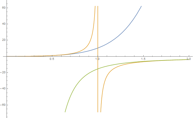
Note: Depending on whether the objects are inside or outside the torus, you should use different approximations for the torus' gravitational field, which can be found in the link mentioned above.

In[26]:= Simplify[
 Series[1 x Integrate[(Cos[t] - x)/(1 - 2 x Cos[t] + (x)^2)^1.5, {t, 
     0, 2 Pi}], {x, 0, 6}], x < 1]

Out[26]= SeriesData[x, 0, {3.1415926535897927`, 0., \
3.5342917352885173`, 0., 3.6815538909255383`}, 2, 7, 1]

In[29]:= Simplify[
 Series[1/x Integrate[(Cos[t] - 1/x)/(1 - 
      2/x Cos[t] + (1/x)^2)^1.5, {t, 0, 2 Pi}], {x, 0, 6}], 0 < x < 1]

Out[29]= SeriesData[x, 0, {-6.283185307179585, 0., \
-4.712388980384691, 0., -4.417864669110656}, 1, 7, 1]

In[24]:= Plot[{3.1415926535897927` x^2 + 3.5342917352885173` x^4 + 
   3.6815538909255383` x^6, 
  x NIntegrate[(Cos[t] - x)/(1 - 2 x Cos[t] + x^2)^1.5, {t, 0, 
     2 Pi}], -6.283185307179585` /x - 4.712388980384691` (1/x)^3 - 
   4.417864669110656` (1/x)^5}, {x, 0, 2}]

enter image description here

$\endgroup$
3
  • $\begingroup$ First of all, I certainly appreciate the effort gone into this. If I make a VectorPlot3D[] of the acceleration for {fx,fy,fz} = G m3 F[EuclideanDistance[{x1, y1, z1}, {x3, y3, z3}], AU] (Normalize[{x1, y1, z1} - {x3, y3, z3}][[{1,2,3}]]) /. {x3 -> 0, y3 -> 0, z3 -> 0}; VectorPlot3D[{fx, fy, fz}, {x1, -a AU, a AU}, {y1, -a AU, a AU}, {z1, -a/2 AU, a/ AU}, BoxRatios -> {1, 1, 0.5}] For any a gives the same result, of radiating outward horizontally, which isn't an expected result. $\endgroup$
    – Feyre
    Commented Jul 20, 2016 at 10:58
  • $\begingroup$ Please Notice that the Approximation that I've made was for an object inside the asteroid belt. As you can see you should use another form of approximation for the objects outside the torus: $\endgroup$
    – Siav Josep
    Commented Jul 20, 2016 at 12:17
  • $\begingroup$ Alright, I can't verify now, will accept once I have worked this through. $\endgroup$
    – Feyre
    Commented Jul 20, 2016 at 12:59

Your Answer

By clicking “Post Your Answer”, you agree to our terms of service and acknowledge you have read our privacy policy.

Not the answer you're looking for? Browse other questions tagged or ask your own question.