Exponential fitting - isn't actually a BUG there?

Question

There are many questions on this site about wrong exponential fitting in Mathematica but no one considers this well-known problem as a potential bug. Usually people suggest well-known workarounds allowing to obtain expected results but they don't investigate the source of the problem. My recent attempt to understand the situation lead me to conclusion that there is a bug in FindFit and FindMinimum related to exponential fitting.

Let us take a simple dataset and try to fit it to the exponential model:

data = {{0, 20}, {20, 10}, {40, 5}, {60, 2.5}, {80, 1.25}};
fit1 = FindFit[data, a*Exp[b*x], {a, b}, x, EvaluationMonitor :> Print[{a, b}]]

{1.,1.}

{0.,1.}

 {a -> 0., b -> 1.}

Isn't the observed behavior already strange? Only two points are taken and then the last of them is returned as the minimum without any messages! It is easy to see that the returned solution is completely wrong and the correct solution can be obtained with Method -> NMinimize:

fit2 = FindFit[data, a*Exp[b*x], {a, b}, x, Method -> NMinimize]
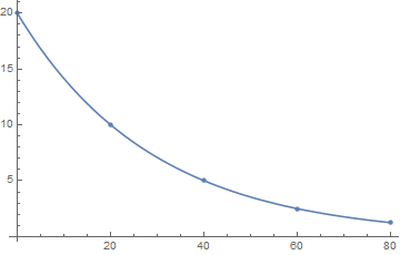
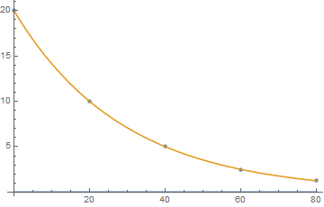
Show[ListPlot[data], Plot[Evaluate[a*Exp[b*x] /. {fit1, fit2}], {x, 0, 80}]]

{a -> 20., b -> -0.0346574}

But WHY the default method (which is "LevenbergMarquardt") gives wrong result? Maybe there actually is a local minimum with zero gradient? Let us check the gradient of the Sum of Squared Residuals (which is the function minimized by FindFit; SSR below) at the points checked by FindFit:

Clear[a, b, x]
model[x_] := a*Exp[b*x];
resudual[{x_, y_}] := y - model[x];
residuals = Table[resudual[point], {point, data}];
SSR = Total[residuals^2];
gradientVector = D[SSR, {{a, b}}];
gradientVector /. {{a -> 1., b -> 1.}, {a -> 0., b -> 1.}}

{{6.1397*10^69, 4.91176*10^71}, {-1.38516*10^35, 0.}}

The gradient is HUGE in absolute value at both points checked by FindFit but it returns the last of them as the solution without any messages! FindMinimum behaves identically:

FindMinimum[SSR, {a, b}]

{532.813, {a -> 0., b -> 1.}}

Can anyone explain this behavior (I'm not looking for a workaround, I'm looking for an explanation)? Is this a bug?

Answer 1

This looks like a numerical precision issue. Various approaches that precisely address this, all yield the same, correct solution:

Scaling of the x values:

data = {{0, 20}, {20, 10}, {40, 5}, {60, 2.5}, {80, 1.25}};
{xmin, xmax} = MinMax[data[[All,1]]];
data2 = {Rescale[data[[All, 1]]], data[[All, 2]]} // Transpose;
fit1 = FindFit[data2, a*Exp[b*x], {a, b}, x];
Show[ListPlot[data], 
 Plot[a*Exp[b*Rescale[x, {xmin, xmax}]] /. fit1, {x, 0, 80}]]

Exact numbers:

data = {{0, 20}, {20, 10}, {40, 5}, {60, 25/10}, {80, 125/100}};
fit1 = FindFit[data, a*Exp[b*x], {a, {b, -1}}, x]
Show[ListPlot[data], Plot[Evaluate[a*Exp[b*x] /. fit1], {x, 0, 80}]]
(* {a -> 20., b -> -0.0346574} *)

Arbitrary precision numbers:

data = {{0, 20}, {20, 10}, {40, 5}, {60, 2.5`500}, {80, 1.25`500}};
fit1 = FindFit[data, a*Exp[b*x], {a, {b, -1}}, x]

(*{a -> 19.9999999999999999999999999999999999999999999999999999999999999\
9999999999999999999999999999999999999999999999999999999999999999999999\
9999999999999999999999999999999999999999999999999999999999999999999999\
9999999999999999999999999999999999999999999999999999999999999999999999\
9999999999999999999999999778047394451665874718796271036850250884181562\
4585573342662728816721398861154072988885262039061332356855851201362915\
7164434036094129659039810884391575813515277252575297641755499155092912\
05514394088532664, 
 b -> -0.0346573590279972654708616060729088284037750067180127627060340\
0047466968109848473578029316634982093437710007405102853428668427601178\
7906527851633537581753798096536378541418571759515351931194583673556167\
5057682248977619560237586340787466032577762367069762941475226503547663\
1833213270521195789074760212376423504358288082923157416807773455937594\
8730959223814463379866456988534715801639211694432455726463474594405763\
7863828006795995086471222261587769767698218890439528263697455009896183\
99973828035023378735} *)

Answer 2

I am one of the many that does not consider this a bug as it is shared by probably the majority of statistical packages. (But there certainly is room for improvement in terms of warnings that could be given.)

Iterative procedures work great if the starting values are close enough to the final values. When one doesn't know the final result this requirement can be a bit daunting.

However, there are things that one can do to reduce the number of such failures.

(1) Find out what starting values are used by the fitting function. For this function Mathematica uses 1.0 as the starting value for all parameters. Consider the part of the function Exp[b*x]. With b = 1.0 and x = 80. Exp[1.0*80] = 5.54062*10^34. At the other end of the data there is x = 0 which gives Exp[1.0*0] = 1.0. This range of numerical values is bound to cause trouble.

(2) Standardize the independent variables. You can (a) subtract the mean and divide by the standard deviation or range, or (b) subtract the minimum value from each value if there are numerous superflous digits (as in geographical UTM units), or (c) divide by a power of 10 to get all values between 0 and 10. (And one should determine that doing so doesn't change the basic equation.)

One should also consider whether linearizing the equation might help in numerical stability and have the distribution of the residuals match the assumptions. (In other words, fitting y = logA + b * x + error.)

For this particular dataset one could divide the x values by 10 and everything works:

fit2 = FindFit[data, a*Exp[b*x/10], {a, b}, x, 
  EvaluationMonitor :> Print[{a, b}]]
(* {1.`,1.`}
{0.041318727177279246`,0.9948817357756237`}
{0.04283227733515496`,0.8664735714509461`}
{0.08908837807900087`,0.6097184994465492`}
{0.3761606155865537`,0.09730611472542439`}
{5.268929789483257`,-0.796208595732955`}
{13.173242486336434`,-0.5173835399541626`}
{19.927460536660046`,-0.17029501801604285`}
{19.503033453296695`,-0.2801530807616852`}
{19.9570169999364`,-0.33847226843982786`}
{19.999529625704145`,-0.3464506437357793`}
{19.999999896325985`,-0.3465735609902636`}
{19.999999999999993`,-0.3465735902799709`} *)

Update

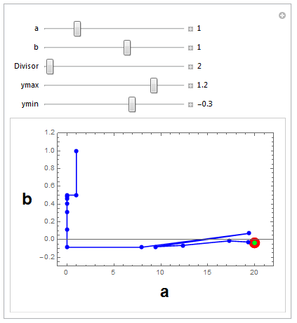
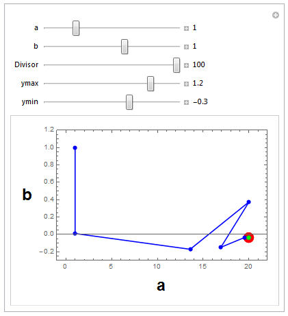
Maybe to show what is going on (which I'm still claiming is a scaling issue) is the following:

Manipulate[
 (* Determine fit *)
 fit = Reap[
   FindFit[data, a*Exp[b*x/k], {{a, aa}, {b, bb}}, x, 
    EvaluationMonitor :> Sow[{a, b}]]];

 (* Adjust estimate of b to be on original scale *)
 fit[[2, 1, All, 2]] = fit[[2, 1, All, 2]]/k;

 (* Plot results *)
 ListPlot[{{{20, -0.0346754}}, Prepend[fit[[2, 1]], {aa, bb}], 
   Prepend[fit[[2, 1]], {aa, bb}], {{a, b/k}} /. fit[[1]]}, 
  PlotStyle -> {{Red, PointSize[0.05]}, {Blue, 
     PointSize[0.02]}, {Blue, PointSize[0.02]}, {Green, 
     PointSize[0.02]}},
  Joined -> {False, True, False}, AxesOrigin -> {-1, 0}, 
  PlotRange -> {{-1, 22}, {ymin, ymax}},
  Frame -> True, 
  FrameLabel -> {Style["a", Large, Bold, Black], 
    Rotate[Style["b", Large, Bold, Black], -\[Pi]/2]}],

 (* Controls *)
 {{aa, 1, "a"}, -5, 22, Appearance -> "Labeled"},
 {{bb, 1, "b"}, -0.5, 2, Appearance -> "Labeled"},
 {{k, 2, "Divisor"}, 0.1, 100, Appearance -> "Labeled"},
 {{ymax, 1.2}, 0, 1.5, Appearance -> "Labeled"},
 {{ymin, -0.3}, -1, 0.1, Appearance -> "Labeled"},
 TrackedSymbols :> {aa, bb, k, ymin, ymax},
 Initialization :> (data = {{0, 20}, {20, 10}, {40, 5}, {60, 
      2.5}, {80, 1.25}})]

I believe this shows that without scaling of the x values, the search algorithm is dominated by looking for good values of b and essentially ignoring a until b is found. A more stable search occurs when successive points move a bit in both a and b directions.

Here is where the scaling factor (i.e., what we divide b by) is 2:

Now with the scaling factor being 100:

Answer 3

In the comments I supposed that the reason why the algorithm stops is obtaining zero derivative with respect to b at the point {a, b} = {0., 1.} returned as the minimum. Let us check this statement by perturbing the actual Jacobian a little bit in order to make all the derivatives non-zero.

Proceeding from the code in the question, we find the Jacobian and feed it to FindMinimum as described here:

jacobianMatrix = D[residuals, {{a, b}}];

FindMinimum[, {a, b}, 
 Method -> {"LevenbergMarquardt", "Residual" :> Sqrt[2] residuals, 
   "Jacobian" :> (Sqrt[2] jacobianMatrix)}]

{532.813, {a -> 0., b -> 1.}}

The result is exactly the same as with automatic Jacobian:

% === FindMinimum[SSR, {a, b}]

True

Now we add a tiny constant perturbation to the Jacobian:

FindMinimum[, {a, b}, 
 Method -> {"LevenbergMarquardt", "Residual" :> Sqrt[2] residuals, 
   "Jacobian" :> (Sqrt[2] jacobianMatrix - 10^-150)}]

FindMinimum::cvmit: Failed to converge to the requested accuracy or precision within 100 iterations. >>

{531.25, {a -> 3.37441*10^-35, b -> 0.994968}}

The situation has moved forward! Let us increase the number of iterations:

FindMinimum[SSR, {a, b}, 
 Method -> {"LevenbergMarquardt", "Residual" :> Sqrt[2] residuals, 
   "Jacobian" :> (Sqrt[2] jacobianMatrix - 10^-150)}, MaxIterations -> 10000]

{8.39587*10^-20, {a -> 20., b -> -0.0346574}}

We have got the correct solution!

Now let us investigate it a little deeper and create a "smarter" perturbation which will be non-zero only at the second evaluation of the Jacobian:

counter = 0;
myJacobian[count_] := If[count == 2, jacobianMatrix + 10^-150, jacobianMatrix];

FindMinimum[SSR, {a, b}, 
 Method -> {"LevenbergMarquardt", "Residual" :> Sqrt[2] residuals, 
   "Jacobian" :> (Sqrt[2] myJacobian[++counter])}, MaxIterations -> 10000]

{5.29677*10^-25, {a -> 20., b -> -0.0346574}}

It is easy to check that if we make the perturbation non-zero at any other evaluation except the second, we obtain incorrect solution. So it is the second value of the Jacobian what is the stumbling block for the algorithm:

jacobianMatrix /. {a -> 0.`, b -> 1.`}

{{-1, 0}, {-4.85165*10^8, 0.}, {-2.35385*10^17, 0.}, {-1.14201*10^26, 
  0.}, {-5.54062*10^34, 0.}}

One can see that all derivatives with respect to b are zero (as expected for a = 0).

Now let us make all the derivatives with respect to b zero at some arbitrary step of the algorithm (but at the second step we will keep the perturbation):

counter = 0;
myJacobian[count_] := 
  Which[count == 2, jacobianMatrix + 10^-150, count == 10, 
   jacobianMatrix*ConstantArray[{1, 0}, 5], True, jacobianMatrix];

FindMinimum[SSR, {a, b}, 
 Method -> {"LevenbergMarquardt", "Residual" :> Sqrt[2] residuals, 
   "Jacobian" :> (Sqrt[2] myJacobian[++counter])}, MaxIterations -> 10000]
counter

{531.25, {a -> 1.1088*10^-31, b -> 0.89375}}

11

Experimentation shows that the algorithm always stops after the step when it gets the Jacobian with zero derivatives with respect to b (but it won't stop if at least for one data point this derivative is non-zero). From the other side, if we make at some step zero derivatives with respect to a, it does not stop the algorithm:

counter = 0;
myJacobian[count_] := 
  Which[count == 2, jacobianMatrix + 10^-150, count == 1000, 
   jacobianMatrix*ConstantArray[{0, 1}, 5], True, jacobianMatrix];

FindMinimum[SSR, {a, b}, 
 Method -> {"LevenbergMarquardt", "Residual" :> Sqrt[2] residuals, 
   "Jacobian" :> (Sqrt[2] myJacobian[++counter])}, MaxIterations -> 10000]
counter

{1.97215*10^-31, {a -> 20., b -> -0.0346574}}

4119

Of course I still have not explained what is so special about zero derivatives with respect to b. I still feel this behavior as a bug or at least significant imperfection of current implementation.