89
$\begingroup$

Background: I use code from An Efficient Test For A Point To Be In A Convex Polygon Wolfram Demonstration to check if a point ( mouse pointer ) is in a ( convex ) polygon. Clearly this code fails for non-convex polygons.

Question: I am looking for an efficient routine to check if a 2D-point is in a polygon.

$\endgroup$
9
  • 1
    $\begingroup$ I don't believe Mathematica has a build-in function for this. You could build your own in which case this is a good starting point: point in polygon $\endgroup$
    – jVincent
    Commented Aug 14, 2012 at 8:39
  • $\begingroup$ Perhaps this answer by Heike? $\endgroup$
    – kglr
    Commented Aug 14, 2012 at 8:49
  • 2
    $\begingroup$ It's pretty depressing that you already accepted an answer before I posted mine, but I posted anyway. :-/ $\endgroup$
    – Mr.Wizard
    Commented Aug 14, 2012 at 10:02
  • 4
    $\begingroup$ The best answer to this question depends on the intended use and other constraints. The most important determinants are (1) whether this will be a one-off test or if many points will be tested for a given polygon; (2) where the points are likely to fall; and (3) whether the test needs to be absolutely accurate. Except for the one-off accurate test, by far the fastest method--and one not yet offered in any answer--is to rasterize the polygon's interior, probe the raster at the point's location (a $O(1)$ operation), and revert to a more expensive test only if the probe is inconclusive. $\endgroup$
    – whuber
    Commented Aug 14, 2012 at 17:52
  • 4
    $\begingroup$ The various responses are quite good. That said, if you have to test many points and the polygon has many vertices, the method indicated at this link should be fairly efficient. forums.wolfram.com/mathgroup/archive/2009/Feb/msg00519.html $\endgroup$ Commented Aug 14, 2012 at 21:10

11 Answers 11

56
$\begingroup$

Using the function winding from Heike's answer to a related question

 winding[poly_, pt_] := 
 Round[(Total@ Mod[(# - RotateRight[#]) &@(ArcTan @@ (pt - #) & /@ poly), 
  2 Pi, -Pi]/2/Pi)]

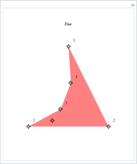
to modify the test function in this Wolfram Demonstration by R. Nowak to

testpoint[poly_, pt_] := 
Round[(Total@ Mod[(# - RotateRight[#]) &@(ArcTan @@ (pt - #) & /@ poly), 
    2 Pi, -Pi]/2/Pi)] != 0

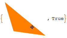
gives

enter image description here

Update: Full code:

Manipulate[With[{p = Rest@pts, pt = First@pts},
   Graphics[{If[testpoint[p, pt], Pink, Orange], Polygon@p},
   PlotRange -> 3 {{-1, 1}, {-1, 1}},
   ImageSize -> {400, 475},
   PlotLabel -> Text[Style[If[testpoint[p, pt], "True ", "False"], Bold, Italic]]]],
 {{pts, {{0, 0}, {-2, -2}, {2, -2}, {0, 2}}}, 
 Sequence @@ (3 {{-1, -1}, {1, 1}}), Locator, LocatorAutoCreate -> {4, Infinity}},
 SaveDefinitions -> True,   
 Initialization :> {
 (* test if point pt inside polygon poly *)
    testpoint[poly_, pt_] := 
    Round[(Total@ Mod[(# - RotateRight[#]) &@(ArcTan @@ (pt - #) & /@ poly), 
       2 Pi, -Pi]/2/Pi)] != 0 } ]

Update 2: An alternative point-in-polygon test using yet another undocumented function:

 testpoint2[poly_, pt_] := Graphics`Mesh`InPolygonQ[poly, pt]

 testpoint2[{{-1, 0}, {0, 1}, {1, 0}}, {1/3, 1/3}]
 (*True*)
 testpoint2[{{-1, 0}, {0, 1}, {1, 0}}, {1, 1}]
 (*False*)
$\endgroup$
19
  • $\begingroup$ Looks great! I'll try to implement this in my app and let you know asap. Thank you very much. $\endgroup$ Commented Aug 14, 2012 at 9:14
  • $\begingroup$ The testpoint function is a beauty. I would give a bonus if possible, I'll do a fast accept, instead. Thanks kguler $\endgroup$ Commented Aug 14, 2012 at 9:57
  • 1
    $\begingroup$ This doesn't work for self-intersecting polygons, but you could use PolygonTessellation from the package linked in my answer to pre-process. +1 $\endgroup$
    – Mr.Wizard
    Commented Aug 14, 2012 at 10:39
  • 1
    $\begingroup$ @matheorem, i used ??*`*PointWindingNumber* $\endgroup$
    – kglr
    Commented Dec 3, 2014 at 2:02
  • 1
    $\begingroup$ @matheorem There is no Graphics`Mesh`* context in v10. You must be seeing it because a symbol was created in that context when you tried kguler's answer or mine (which didn't work). Try again in a fresh session and you won't see it. $\endgroup$
    – rm -rf
    Commented Dec 3, 2014 at 14:07
85
$\begingroup$

The undocumented Graphics`PolygonUtils`PointWindingNumber (if you're on versions < 10, use Graphics`Mesh`PointWindingNumber) does exactly this — it gives you the winding number of a point. A point lies inside the polygon if and only if its winding number is non-zero.

Using this, you can create a Boolean function to test if a point is inside the polygon

inPolyQ[poly_, pt_] := Graphics`PolygonUtils`PointWindingNumber[poly, pt] =!= 0

(* Examples *)
inPolyQ[{{-1, 0}, {0, 1}, {1, 0}}, {1/3, 1/3}]
(* True *)
inPolyQ[{{-1, 0}, {0, 1}, {1, 0}}, {1, 1}]
(* False *)

Or, you can use the aptly named Graphics`PolygonUtils`InPolygonQ which has the same 2-argument syntax and is a predicate.

$\endgroup$
7
  • 7
    $\begingroup$ One could also use Graphics`Mesh`InPolygonQ, which has the same 2 argument syntax as Graphics`Mesh`PointWindingNumber. The former also takes a Method option, which I haven't explored yet... $\endgroup$
    – rm -rf
    Commented Aug 14, 2012 at 16:37
  • $\begingroup$ I implement windnig number myself but this is better, I bet faster. A newbie Q: how can I see how this functions is coded, its syntax? I can see there's also PolygonWindingNumber in ver. 9 and I'd like to see what it does if I can. $\endgroup$
    – BoLe
    Commented Apr 19, 2013 at 8:16
  • 2
    $\begingroup$ @BoLe Unfortunately, it doesn't look like the code for this one is accessible... In general, the tighter a function's integration with the kernel, the harder it is (almost impossible) to read its definitions (e.g. Pick, Cases, etc.). You can, however, read them for several other functions that are implemented in top level Mathematica. Usually all that one needs to do is to clear the attributes, read the definitions and follow the rabbit hole of internal definitions. However, instead of that, I'll recommend this answer. Prepare to be amazed :) $\endgroup$
    – rm -rf
    Commented Apr 19, 2013 at 13:41
  • $\begingroup$ @rm-rf As I tested it, this undocumented Graphics`Mesh`PointWindingNumber is not working in V10, so maybe undocumented function is dangerous? $\endgroup$
    – matheorem
    Commented Dec 3, 2014 at 0:43
  • 1
    $\begingroup$ @rm-rf Thank you! kguler told me using ??*`*PointWindingNumber* could see which package that PointWindingNumber belongs to. But I found V10 gives both Mesh and PolygonUtils, you can see here imgur.com/bCIANiR, then why Mesh didn't work any more? $\endgroup$
    – matheorem
    Commented Dec 3, 2014 at 6:35
28
$\begingroup$

Sometimes speed is an issue if there are many polygons and or many points to check. There is an excellent reference on this issue under http://erich.realtimerendering.com/ptinpoly/ with the main conclusion that the angle summation algorithm should be avoided if speed is the objective.

Below is my Mathematica implementation of the point in polygon problem which appears to be roughly 5x faster than the inPolyQ[] algorithm posted above.

Test case - use triangle

poly = {{-1, 0}, {0, 1}, {1, 0}};

My code implementation

inPoly2[poly_, pt_] := Module[{c, nvert,i,j},
   nvert = Length[poly];
   c = False;
   For[i = 1, i <= nvert, i++,
    If[i != 1, j = i - 1, j = nvert];
    If[(
      ((poly[[i, 2]] > pt[[2]]) != (poly[[j, 2]] > pt[[2]])) && (pt[[
      1]] < (poly[[j, 1]] - 
         poly[[i, 1]])*(pt[[2]] - poly[[i, 2]])/(poly[[j, 2]] - 
          poly[[i, 2]]) + poly[[i, 1]])), c = ! c];
    ];
   c
   ];

An the timing output testing on point {0,0.99}

Timing[t1 = Table[inPolyQ[poly, 0, 0.99], {10000}];]
Timing[t2 = Table[inPoly2[poly, 0, 0.99], {10000}];]

Out[115]= {0.062, Null}
Out[116]= {0.016, Null}

Update Following a suggestion from ruebenko I've now investigated the actual performance of all the different point-in-polygon routines for two specific cases.

Test No1: Simple triangle polyon and testing using 5000 random test points

poly = {{-1, 0}, {0, 1}, {1, 0}};
pts = Partition[RandomReal[{-1, 1}, 10000], 2];
npts = Length@pts;
Print["inPoly2: ", 
 Timing[Table[inPoly2[poly, pts[[i]]], {i, npts}];][[1]]]
Print["testpoint: ", 
 Timing[Table[testpoint[poly, pts[[i]]], {i, npts}];][[1]]]
Print["testpoint2: ", 
 Timing[Table[testpoint2[poly, pts[[i]]], {i, npts}];][[1]]]
Print["inPolyQ: ", 
 Timing[Table[inPolyQ[poly, pts[[i]]], {i, npts}];][[1]]]
Print["InsidePolygonQ: ", 
 Timing[Table[InsidePolygonQ[poly, pts[[i]]], {i, npts}];] [[1]]]
Print["inPolyQ2: ", 
 Timing[Table[
     inPolyQ2[poly, pts[[i, 1]], pts[[i, 2]]], {i, npts}];][[1]]]

with the following results

inPoly2: 0.202
testpoint: 0.25
testpoint2: 0.016
inPolyQ: 0.015
InsidePolygonQ: 12.277
inPolyQ2: 0.032

Test No2: Very complicated polygon. The main CountryData[] polygon for Canada has over 10 000 vertices and a fairly complex shape. I've focused on the fastest routines and excluded the InsidePolygonQ[] routine in this case and used 200 test points.

p = CountryData["Canada", "Polygon"][[1, 1]];
poly = {Rescale[p[[All, 1]], {Min@#, Max@#} &@p[[All, 1]], {-1, 1}],
    Rescale[p[[All, 2]], {Min@#, Max@#} &@p[[All, 2]], {-1, 1}]} // 
   Transpose;
pts = Partition[RandomReal[{-1, 1}, 400], 2];
npts = Length@pts;
Print["inPoly2: ", 
 Timing[Table[inPoly2[poly, pts[[i]]], {i, npts}];][[1]]]
Print["testpoint: ", 
 Timing[Table[testpoint[poly, pts[[i]]], {i, npts}];][[1]]]
Print["testpoint2: ", 
 Timing[Table[testpoint2[poly, pts[[i]]], {i, npts}];][[1]]]
Print["inPolyQ: ", 
 Timing[Table[inPolyQ[poly, pts[[i]]], {i, npts}];][[1]]]
Print["inPolyQ2: ", 
 Timing[Table[
 inPolyQ2[poly, pts[[i, 1]], pts[[i, 2]]], {i, npts}];][[1]]]

with the following results

inPoly2: 8.237
testpoint: 11.295
testpoint2: 0.156
inPolyQ: 0.436
inPolyQ2: 0.078

My verdict: There is an astonishing 3 orders of magnitude difference in the performance of the different routines. InsidePolygonQ[] while mathematically elegant, is very slow. It pays to use either the undocumented routine for point in polygon in Mathematica, in this case testpoint2[] (with the usual caveats), or the compiled routine inPolyQ2[] which both had excellent performance for both simple and complex test polygons.

$\endgroup$
5
  • $\begingroup$ Mac, thanks for contributing. Looks interesting! I recommend that you localize i and j. $\endgroup$
    – Mr.Wizard
    Commented Aug 14, 2012 at 11:26
  • $\begingroup$ Thanks for the suggestion - have updated the code accordingly with i and j now localised. $\endgroup$
    – Mac
    Commented Aug 14, 2012 at 11:48
  • $\begingroup$ I'd replace the For[] with a Do[] myself... $\endgroup$ Commented Aug 14, 2012 at 13:21
  • 2
    $\begingroup$ @Mac, you could use a slightly larger polygon (e.g. the polygon from a country from CountryData) and some Random points (with a SeedRandom) and see how that performs ;-) $\endgroup$
    – user21
    Commented Aug 14, 2012 at 14:21
  • $\begingroup$ @mac p is not right, should be p = CountryData["Canada", "Polygon"][[1, 1,25]];. Because there are 25 parts in Canada. The main part is 25th. Tested in V10 $\endgroup$
    – matheorem
    Commented Oct 11, 2015 at 6:59
27
$\begingroup$

The second "Neat Example" in the documentation for SmoothKernelDistribution contains this compiled function:

(* A region function for a bounding polygon using winding numbers: *)

inPolyQ = 
  Compile[{{polygon, _Real, 2}, {x, _Real}, {y, _Real}}, 
   Block[{polySides = Length[polygon], X = polygon[[All, 1]], 
     Y = polygon[[All, 2]], Xi, Yi, Yip1, wn = 0, i = 1}, 
    While[i < polySides, Yi = Y[[i]]; Yip1 = Y[[i + 1]]; 
     If[Yi <= y, 
      If[Yip1 > y, Xi = X[[i]]; 
        If[(X[[i + 1]] - Xi) (y - Yi) - (x - Xi) (Yip1 - Yi) > 0, 
         wn++;];];, 
      If[Yip1 <= y, Xi = X[[i]]; 
        If[(X[[i + 1]] - Xi) (y - Yi) - (x - Xi) (Yip1 - Yi) < 0, 
         wn--;];];]; i++]; ! wn == 0]];

Edit

As Mr Wizard discovered, the function above does not work unless the last point in the polygon is the same as the first. Here is a version which doesn't have that limitation, and as a bonus is slightly faster.

Edit 2 : Code tweaked for more speed (thanks again to Mr. Wizard)

inPolyQ2 = Compile[{{poly, _Real, 2}, {x, _Real}, {y, _Real}},
   Block[{Xi, Yi, Xip1, Yip1, u, v, w},
    {Xi, Yi} = Transpose@poly;
    Xip1 = RotateLeft@Xi;
    Yip1 = RotateLeft@Yi;
    u = UnitStep[y - Yi];
    v = RotateLeft@u;
    w = UnitStep[-((Xip1 - Xi) (y - Yi) - (x - Xi) (Yip1 - Yi))];
    Total[(u (1 - v) (1 - w) - (1 - u) v w)] != 0]];

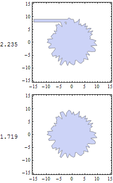
Comparison showing that the defect in the original is not present in the new code:

poly = Table[RandomReal[{7, 10}] {Sin[th], Cos[th]}, {th, 2 Pi/100, 2 Pi, 2 Pi/100}];

Grid[Timing[RegionPlot[#[poly, x, y], {x, -15, 15}, {y, -15, 15}, 
     PlotPoints -> 100]] & /@ {inPolyQ, inPolyQ2}]

enter image description here

$\endgroup$
3
  • $\begingroup$ Damn, I was about to post this myself... :D $\endgroup$ Commented Aug 14, 2012 at 10:22
  • $\begingroup$ For speed I would try: Xip1 = RotateLeft@Xi; Yip1 = RotateLeft@Yi; and Total[u (1 - v) (1 - w) - (1 - u) v w] $\endgroup$
    – Mr.Wizard
    Commented Aug 15, 2012 at 0:22
  • $\begingroup$ I'll just note that inPolyQ2 is exactly what you'll end up with if you try to vectorize Sunday's implementation of the winding number algorithm. $\endgroup$ Commented Jan 15, 2017 at 14:13
27
$\begingroup$

Another approach to this problem is computing the winding number by integrating $1/z$ centered on the point of interest along the contour of the polygon in the complex plane. Sure this isn't exactly efficient, but still I think it's nice to see this working in action. And since complex integration is feasible in Mathematica, I just tried :)

PointToComplex[{x_, y_}] := x + I y
Windingnumber[polygon_, point_] := Module[{wn,z},
  Off[NIntegrate::ncvb, NIntegrate::slwcon]; 
  wn = Round@
    Re@Chop[1/(2 π I)
        NIntegrate[1/(z - PointToComplex[point]), 
        Evaluate@{z, Sequence @@ (PointToComplex /@ Append[#, #[[1]]]&[polygon])}]];
  On[NIntegrate::ncvb, NIntegrate::slwcon];
  wn
  ]
InsidePolygonQ[polygon_, point_] := Windingnumber[polygon, point] != 0
$\endgroup$
5
  • 1
    $\begingroup$ You can use Complex @@@ r in place of PointToComplex /@ polygon, etc., I believe. $\endgroup$
    – Mr.Wizard
    Commented Aug 14, 2012 at 13:40
  • 2
    $\begingroup$ @Mr. Wizard, if they're explicitly numbers (i.e. passes NumberQ[] but not NumericQ[]). Complex @@ {1, Pi} won't work, for instance. $\endgroup$ Commented Aug 14, 2012 at 15:34
  • 1
    $\begingroup$ I think this is the first time that code has made me laugh (at least for positive reasons), so +1! $\endgroup$
    – acl
    Commented Aug 14, 2012 at 15:57
  • $\begingroup$ @Mr.Wizard Thanks for the hint! Applying Complex didn't cross my mind when i wrote the code. @J.M. interesting detail, never looked at how Mathematica handles complex number representation! $\endgroup$ Commented Aug 15, 2012 at 8:32
  • $\begingroup$ @acl Ha, glad to hear that :) was definitely worth posting then ;) $\endgroup$ Commented Aug 16, 2012 at 22:48
23
$\begingroup$

You could use this package to triangulate your polygon, and then use this barycentric formula on each of the triangles.

inside[{{x1_, y1_}, {x2_, y2_}, r3 : {x3_, y3_}}, r : {_, _}] :=
  # >= 0 && #2 >= 0 && # + #2 < 1 & @@
    LinearSolve[{{x1 - x3, x2 - x3}, {y1 - y3, y2 - y3}}, r - r3]

Example for a single triangle:

tri = {{13.2, 11.9}, {10.3, 12.3}, {9.5, 14.9}};

{
 LocatorPane[Dynamic @ pt, Graphics @ {Orange, Polygon@tri}],
 Dynamic @ inside[tri, pt]
}

Mathematica graphics

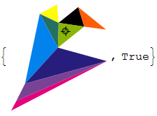
Example for a polygon:

<< PolygonTriangulation`SimplePolygonTriangulation`

poly = {{4.4, 14}, {6.7, 15.25}, {6.9, 12.8}, {9.5, 14.9}, {13.2, 
    11.9}, {10.3, 12.3}, {6.8, 9.5}, {13.3, 7.7}, {0.6, 1.1}, {1.3, 
    2.4}, {2.45, 4.7}};

tris = poly[[#]] & /@ SimplePolygonTriangulation[poly];

colors = MapIndexed[{ColorData[3] @ #2[[1]], Polygon@#} &, tris];

DynamicModule[{pt},
 {LocatorPane[Dynamic[pt], colors // Graphics],
  Or @@ (inside[#, pt] & /@ tris) // Dynamic}
]

Mathematica graphics

$\endgroup$
2
  • 3
    $\begingroup$ Didn't notice until now, but Inverse[{{x1 - x3, x2 - x3}, {y1 - y3, y2 - y3}}].(r - r3) is better done as LinearSolve[{{x1 - x3, x2 - x3}, {y1 - y3, y2 - y3}}, r - r3]. $\endgroup$ Commented Aug 31, 2012 at 15:10
  • $\begingroup$ @J.M. good to know; thanks! $\endgroup$
    – Mr.Wizard
    Commented Sep 1, 2012 at 19:57
20
$\begingroup$

As per Szabolcs's suggestion:

Version 10 alternatives are RegionMember and Element, but the latter is unreasonably slow.

A drop in alternative

RegionMember[reg] returns a RegionMemberFunction[...] that can be applied repeatedly to different points.

(* Memoizing the RegionMemberFunction[...] for a given polygon *)
inPolyQHelper[poly_] := inPolyQHelper[poly] = RegionMember[Polygon@poly];
inPolyQ[poly_, pt_] := inPolyQHelper[poly]@pt

A faster alternative

RegionMember also accepts a list of points to be tested!

RegionMember[Polygon@list, data]

Benchmarks

data = Table[{RandomReal[{-10, 10}], RandomReal[{-10, 10}]}, {i, 1, 1000000}];
list = {{0.5735,5.274},{-4.961,2.333},<<10>>,{-1.662,-0.1829}}; 

(* Compiled version from @Simon Wood's answer *) 
inPolyQSimonWoods[list, Sequence @@ #] & /@ data // AbsoluteTiming // First
(* 11.465298 *)

(* The drop-in RegionMember replacement *)
inPolyQ[list, #] & /@ data // AbsoluteTiming // First
(* 2.994139 *)

(*The fast replacement*))
RegionMember[Polygon@list, data] // AbsoluteTiming // First
(* 0.399948 *)

Just for the record, Element[#, Polygon @ list] /@ data takes 13 seconds with only 100 points.

$\endgroup$
1
  • $\begingroup$ I wish I could vote more. I think RegionMember is by far the fastest based on my test. Who stands with me ! I wish you could add a "Canada test" as Daniel Lichtblau has done. That will better show the power of RegionMember when dealing with complex polygons and lots of points. With a pregenerated RegionFunction at first, RegionMember beats other method badly. $\endgroup$
    – matheorem
    Commented Oct 11, 2015 at 10:20
18
$\begingroup$

Since someone dragged in Canada...

Here is the code from a MathGroup post I had referenced. I have modified to compile to C and that speeds it further. The one-off preprocessing does take time but it seems not unreasonable. It takes a list of lists of polygons (so the "region" need not be connected). To account for this I slightly alter the setup from Mac's response.

Preprocessing the polygon:

getSegsC = 
  Compile[{{j, _Integer}, {minx, _Real}, {len, _Real}, {eps, _Real}, \
{segs, _Real, 3}}, Module[{lo, hi}, lo = minx + (j - 1)*len - eps;
    hi = minx + j*len + eps;
    Select[segs, 
     Module[{xlo, xhi}, {xlo, xhi} = Sort[{#[[1, 1]], #[[2, 1]]}];
       lo <= xlo <= hi || 
        lo <= xhi <= hi || (xlo <= lo && xhi >= hi)] &]]];

polyToSegmentList[poly_, nbins_] := 
 Module[{xvals, yvals, minx, maxx, miny, maxy, segments, flatsegments,
    segmentbins, xrange, len, eps}, {xvals, yvals} = 
   Transpose[Flatten[poly, 1]];
  {minx, maxx} = {Min[xvals], Max[xvals]};
  {miny, maxy} = {Min[yvals], Max[yvals]};
  segments = Map[Partition[#, 2, 1, {1, 1}] &, poly];
  flatsegments = Flatten[segments, 1];
  xrange = maxx - minx;
  eps = 1/nbins*len;
  len = xrange/nbins;
  segmentbins = 
   Table[getSegsC[j, minx, len, eps, flatsegments], {j, nbins}];
  {{minx, maxx}, {miny, maxy}, segmentbins}]

The actual in-or-out code.

pointInPolygon[{x_, y_}, bins_, xmin_, xmax_, ymin_, ymax_] := 
 Catch[Module[{nbins = Length[bins], bin}, 
   If[x < xmin || x > xmax || y < ymin || y > ymax, Throw[False]];
   bin = Ceiling[nbins*(x - xmin)/(xmax - xmin)];
   If[EvenQ[countIntersectionsC[bins[[bin]], x, y, ymin - 1.]], False,
     True]]]

countIntersectionsC = 
  Compile[{{segs, _Real, 3}, {x, _Real}, {yhi, _Real}, {ylo, _Real}}, 
   Module[{tally = 0, yval, xlo, xhi, y1, y2}, 
    Do[{{xlo, y1}, {xhi, y2}} = segs[[j]];
     If[(x < xlo && x < xhi) || (x > xlo && x > xhi), Continue[]];
     yval = y1 + (x - xlo)/(xhi - xlo)*(y2 - y1);
     If[ylo < yval < yhi, tally++];, {j, Length[segs]}];
    tally]];

The mainland of Canada will be the test again. As in Mac's example I rescale so coordinates are all between -1 and 1. This means I really don't need the x/ymin/max stuff but I opted to keep that in.

p = CountryData["Canada", "Polygon"][[1, 1]];
poly = {Transpose[{Rescale[
      p[[All, 1]], {Min@#, Max@#} &@p[[All, 1]], {-1, 1}], 
     Rescale[p[[All, 2]], {Min@#, Max@#} &@p[[All, 2]], {-1, 1}]}]};

I'll use 1000 bins and do the preprocessing.

nbins = 1000;
Timing[{{xmin, xmax}, {ymin, ymax}, segmentbins} = 
   polyToSegmentList[poly, nbins];]

(* Out[369]= {5.15, Null} *)

For testing I'll take 10000 points.

npts = 10000;
pts = Partition[RandomReal[{-1, 1}, 2*npts], 2];

Timing[
 inout = Map[pointInPolygon[#, segmentbins, xmin, xmax, ymin, ymax] &,
     pts];]

(* Out[402]= {0.37, Null} *)

Visual check:

ListPlot[Pick[pts, inout], Joined -> False]
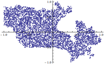
enter image description here

The northeast reminds me a bit of the duck's head seen here. But then...I've always found the Baffin...to be bafflin'.

$\endgroup$
6
  • $\begingroup$ For once Canada is mentioned in another context than exporting cold air down south...(Canadians will know what I mean). $\endgroup$
    – Mac
    Commented Aug 16, 2012 at 9:17
  • $\begingroup$ I don't think we will find a better solution in terms of performance unless perhaps a GPU-solution can be implemented (way above my programming skills in any case). One minor point - you're actually testing 10000 pairs of coordinates (points) not 20000. $\endgroup$
    – Mac
    Commented Aug 16, 2012 at 9:27
  • $\begingroup$ Thanks. I changed from my point generator to yours and failed to catch the effect of the partitioning. Will correct response accordingly.. $\endgroup$ Commented Aug 16, 2012 at 14:33
  • $\begingroup$ Worth pointing out too that the "Canada" polygon example assumes implicitly that each vertex defining the polygon can be connected by a straight line. This has to be a good assumption for such a densely sampled contour. However, for large geographical polygons with few points the connecting edges should be modelled as "great circles". $\endgroup$
    – Mac
    Commented Aug 20, 2012 at 7:25
  • 1
    $\begingroup$ @maththeorem It is very difficult to future-proof code of this sort. It appears that CountryData has changed since this thread was in its infancy. $\endgroup$ Commented Oct 11, 2015 at 16:22
17
$\begingroup$

In version 10 (now available through the Programming Cloud) it is now possible to simply use Element:

For example,

Element[{0,0}, Polygon[{{-1,-1},{-1,1},{1,1},{1,-1}}]]

(* True *)

This works for arbitrary regions in general. Most graphics primitives can be used as regions.

$\endgroup$
3
  • 3
    $\begingroup$ Use RegionMember! It is much faster, specially if you pass the list of points to be tested instead of Map'ing it over them! $\endgroup$
    – Aisamu
    Commented Nov 9, 2014 at 17:28
  • $\begingroup$ @Aisamu Sounds like a much better solution, why don't you post it as an answer? $\endgroup$
    – Szabolcs
    Commented Nov 9, 2014 at 17:32
  • $\begingroup$ I thought there were too many answers already... but I took your advice and just posted it! $\endgroup$
    – Aisamu
    Commented Nov 9, 2014 at 18:05
12
$\begingroup$

Another approach you could use is to draw a line (or define a vector) between a line guaranteed to be outside the polygon and the point you wish to test, then counting the number of line segments of the polygon that intersect with this line. If this number is odd, the point is inside the polygon.

To determine if two line segments intersect, you can use the vector algebra from this SO answer: How do you detect where two line segments intersect?. The short of it is that for any two vectors that intersect, there are two scalars that can be applied, one to each vector, to produce a parallel vector of the exact magnitude needed to reach the intersection. These scalars are a function of the cross product of the vectors. If both scalars are $0 < x < 1$ then this intersection happens within the magnitudes of the original vectors. If $x > 1$ or $x < 0$ for either scalar, they intersect beyond the bounds of the defined vectors, while if $x=0$ the vectors are parallel.

This test should be linear to the number of points defining the polygon (requiring a scan of all points to determine the max X-coord and y-coord to produce a point outside the polygon, and then a scan of all adjacent pairs of points to produce line segments followed by constant-time operations to determine intersection). And, it should work with any 2D polygon you can imagine, no matter how twisted.

$\endgroup$
5
  • $\begingroup$ This is the gist of what I had here. In that case preprocessing, which does take real time, makes the individual queries closer to constant time for "typical" polygons. $\endgroup$ Commented Aug 15, 2012 at 18:45
  • $\begingroup$ the trick in real-world use of this algorithm is the boundary cases - what do you do when the imaginary ray to infinity exactly crosses the intersection of two lines, or is exactly coincident with one of the line segments. $\endgroup$
    – ddyer
    Commented Aug 15, 2012 at 23:22
  • $\begingroup$ @ddyer In actual practice I would probably choose a random direction to approach from. I might also change the binning to use a random orientation rather than horizontal. I might also add a check for hitting a vertex exactly. Depends on how concerned I was about getting a wrong result in a "small" set of cases. $\endgroup$ Commented Aug 16, 2012 at 14:39
  • $\begingroup$ sure, all those things are potential strategies. My point is that a conceptually elegant algorithm has lots of gritty details to be handled if you want to make it work reliably. $\endgroup$
    – ddyer
    Commented Aug 16, 2012 at 18:19
  • 3
    $\begingroup$ @ddyer I actually do this stuff for a living... $\endgroup$ Commented Aug 22, 2012 at 16:36
10
$\begingroup$

Sorry to be late to the party. I'll throw in the following Mathematica implementation of an algorithm by W. Randolph Franklin which I wrote up here a while ago.

The implementation has a number of nice features:

  • Polygon can be closed or not.
  • A point will be inside exactly one member of a polygonal partitioning.
  • No trigonometry, so it's blazing fast.

pnPoly[{testx_, testy_}, pts_List] := Xor @@ ((
  Xor[#[[1, 2]] > testy, #[[2, 2]] > testy] && 
   ((testx - #[[2, 1]]) < (#[[1, 1]] - #[[2, 1]]) (testy - #[[2, 2]])/(#[[1, 2]] - #[[2, 2]]))
  ) & /@ Partition[pts, 2, 1, {2, 2}])
$\endgroup$
5
  • $\begingroup$ The speed will depend linearly on the number of vertices. That is often fine but could be a problem if there are both many vertices and many query points. $\endgroup$ Commented Jan 20, 2014 at 22:53
  • $\begingroup$ @DanielLichtblau: Yes, you are right of course that for a large polygon you want to do something hierarchical along the lines of your answer to get decent scaling. One reason I keep coming back to this implementation is the partitioning guarantee which is critical in much of what I do. $\endgroup$
    – Janus
    Commented Jan 21, 2014 at 8:41
  • $\begingroup$ I had a look at "Insignificance Galore" where it mentions the partitioning guarantee. But I still do not understand what it means. Is it for the case of multiple disconnected polygons? Self-intersecting? Or does it also have meaning in the case of one non-self-intersecting polygon. $\endgroup$ Commented Jan 21, 2014 at 15:29
  • $\begingroup$ A partitioning of a set S is a collection of disjoint subsets of S whose union is S mathworld.wolfram.com/SetPartition.html. The practical problem with partitioning (part of) the plane into polygons is to specify what happens to points on the edges and vertices: it's a lot of tedious details which are usually unimportant from a mathematical point of view (since the combined edges have 0 area), but still needs to be done right for some numerical algorithms to work. $\endgroup$
    – Janus
    Commented Jan 22, 2014 at 8:45
  • $\begingroup$ Okay, thanks for the explanation. I will add that it is also critical, in polynomial irreducibility testing, to know if an exponent vector is or is not a vertex in the convex hull corresponding to a certain a Newton polytope. I can say that numerical convex hull methods have made such determination much more difficult than I would like. So there is at least one math algorithm where this does matter. $\endgroup$ Commented Jan 22, 2014 at 15:51

Your Answer

By clicking “Post Your Answer”, you agree to our terms of service and acknowledge you have read our privacy policy.

Not the answer you're looking for? Browse other questions tagged or ask your own question.