FWHM of an image

Question

What is a resourceful method to calculate FWHM (full width at half the max) of every column in an image. Assuming the image is having a very high resolution for example 1944 x 2592.

Logic so far (applied to every column):

gBW = ImageApply[Mean, zeroS];
data = ImageData[gBW];
datay = data[[All, 1]];

(* For column 1 through 1992 *)
datax = Table[i, {i, 1, Length[data]}];
ListLinePlot[data[[All, 1]], PlotStyle -> Thick,  PlotTheme -> "Detailed"];
(*Colum 1 Peak*)
datay = datay/Max[datay];
L = Length[datay];
Mag = 4;
PP = 2.2;
(*Find the centerindex of maximum*)
CenterIndex = Position[datay, Max[datay]][[1]]; (*Find index of max, first occurence*)
(*start searching lead trail*)
i = 2;
While[Sign[datay[[i]] - 0.5] == Sign[datay[[i - 1]] - 0.5],
      i = i + 1];
Interp = ((0.5 - datay[[i - 1]])/(datay[[i]] - datay[[i - 1]]))
Tlead = datax[[i - 1]] + Interp*(datax[[i]] - datax[[i - 1]])
i = CenterIndex[[1]] + 1

(* Start Searching for the next crossing at center *)
While[Sign[datay[[i]] - 0.5] == Sign[datay[[i - 1]] - 0.5] && (i <= L - 1),
       i = i + 1];
If[i != L, 
    Interp = (0.5 - datay[[i - 1]])/(datay[[i]] - datay[[i - 1]]);
    Ttrail = datax[[i - 1]] + Interp*(datax[[i]] - datax[[i - 1]]);
    FWHM = ((Ttrail - Tlead)/Mag)*PP]

Is there a better approach to do this or a logic to find FWHM along all the columns on the image and plot the same? ( assuming it is going to be a huge number like 2592 columns)

Application: Spectroscopy.

Answer 1

This is a fast discrete approach

i = Import["https://i.sstatic.net/D2GVe.png"];
tid = Transpose[ ImageData[ColorSeparate@ColorConvert[i, "HSB"] // Last]];
nm = Max /@ tid;
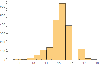
Histogram[2.2/4 MapThread[Count[Sign[#1 - #2/2], 1] &, {tid, nm}]]

Addressing @BlacKow comments below, the following shows that the method works well for this data because all the included segments are contiguous to the maximum:

f[n_] := TakeWhile[Ordering[-tid[[n]]], tid[[n, #]] > Max@tid[[n]]/2 &] // 
                                                       Sort // Differences
fr = f /@ Range@Length@tid;
Times @@ (Flatten@fr)
(* 1 *)

So, the following is "safe" for almost any reasonable dataset:

Histogram[2.2/4 ((f[#] // Split // First // Length) + 1) & /@ Range@Length@tid]

---

Edit

A more careful treatment gives almost the same result:

i = Import["https://i.sstatic.net/D2GVe.png"];
tid = Transpose[ImageData[ColorSeparate@ColorConvert[i, "HSB"] // Last]];
nm = Max /@ tid;
rr = Unitize@MapThread[Sign[#1 - #2/2] + 1 &, {tid, nm}];
mask = {{-1, -1, -1, 1, 1, 1}};
dilated = Dilation[#, 3] & /@ ImageData@
                 HitMissTransform[Image@rr, #, Padding -> 0] & /@ {mask, -mask};
nums = (tid #) & /@ dilated;
ranges = ConstantArray[List /@ Range@Length@First@First@dilated,
                                                     {2, Length@First@dilated}];
lists = MapThread[List, {ranges, nums}, 3];
onlynums = lists /. {{_}, 0.} :> Sequence[];
ints = Transpose@Map[Interpolation, onlynums, {2}];
FWHM = -2.2/4 Subtract @@@ 
    MapThread[
     x /. FindRoot[#1[x] == #2, Evaluate@{x, Sequence @@ #1["Domain"][[1]]}] &, 
              {ints, Transpose@ConstantArray[nm/2, 2]}, 2];

Histogram@FWHM

Answer 2

(Just an extension of belisarius' excellent answer which I have upvoted.)

The physically meaningful approach to the determination of FWHM requires working with actual physical intensity values, not gamma-corrected and artificially deformed intensity values which one gets with the usual photographic cameras generating images in the sRGB colorspace. If it is known that the photo is in the sRGB colorspace, the following conversion function originally published by Jari Paljakka can be used for conversion it into the linear RGB colorspace where channel values represent the actual physical intensity values:

srgb2linear = 
  Compile[{{Csrgb, _Real, 1}}, 
   With[{\[Alpha] = 0.055}, 
    Table[Piecewise[{{C/12.92, C <= 0.04045}, 
                     {((C + \[Alpha])/(1 + \[Alpha]))^2.4, C > 0.04045}}], 
          {C, Csrgb}]], RuntimeAttributes -> {Listable}];

When having actual physical intensity values, it is reasonable to define the overall intensity as a sum of linear intensities for all channels, so belisarius' code can be modifies as follows:

i = Import["https://i.sstatic.net/D2GVe.png"];
tid = Transpose@Total[srgb2linear[ImageData[i, Interleaving -> False]], 1];
nm = Max /@ tid;
Histogram[2.2/4 MapThread[Count[Sign[#1 - #2/2], 1] &, {tid, nm}]]

As one can see, working in the linear color space is crucially important in order to obtain correct estimates of FWHM.