10
$\begingroup$

For example, If a have a curve defined by x^2+y^2=1 and z=0, and some isolated points having z coordinates, Can I construct a 3D surface passed through? It's better if I can change the surface shape by moving the points.

I tried this but failed:

ocir = Table[{Cos[t], Sin[t], 0}, {t, 0, 2 Pi, Pi/8}]  
icir = {{-0.5, 0.6, 0.6}, {0.5, 0.6, 0.6}, {-0.4, -0.8, 0.2}, {0.4, -0.8, 0.2}};
dset = Join[ocir, icir]
Graphics3D[BSplineSurface[dset]]

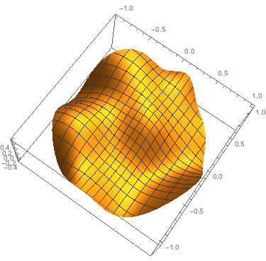
Till now, Öskå's comment is close to my requirement. And MikeLimaOscar gave an interesting extension. I don't know if there are any better solutions.

$\endgroup$
4
  • 3
    $\begingroup$ With ListPlot3D you can have this. $\endgroup$
    – Öskå
    Commented Nov 3, 2014 at 15:21
  • 2
    $\begingroup$ The question is unclear whether the surface is to pass through the points (ListPlot3D) or the points are to control the shape (BSplineSurface). Please clarify. $\endgroup$
    – Michael E2
    Commented Nov 3, 2014 at 17:40
  • $\begingroup$ @MichaelE2,I want the surface to pass through a curve defined by a formula and some isolated points above it. Maybe it's like Concept modeling? It's better if I can change the surface shape by moving the points. $\endgroup$
    – xibinke
    Commented Nov 7, 2014 at 7:56
  • 1
    $\begingroup$ Is the curve the circle defined by $x^2+y^2=$ and $z = 0$? The first equation alone defines a cylindrical surface. Öskå's image seems close to what you want, right? The question is a good question. If you edit it to include the clarification in your comment and about the curve, the community will vote on reopening it. I'm sure they will. $\endgroup$
    – Michael E2
    Commented Nov 7, 2014 at 11:20

3 Answers 3

9
$\begingroup$

Why do it this way? Well, (1) for fun and (2) because Mathematica can. There are infinitely many ways to interpolate a boundary and interior points. One way is to use the FEM functionality to do so. It might be the look the OP wants after all - who knows? :)

We can create an element mesh containing the bounding curve and the xy locations of the points. We can identify the boundary and each point with a marker. For each boundary/point element, we can set a Dirichlet condition with

DirichletCondition[u[x, y] == height, ElementMarker == id]

Then we can interpolate between these heights with any reasonable PDE we like, such as Laplace's equation.

Marking the elements starts with marking the points with pmf; these are pushed to the boundary line elements with bmf. The option "IncludePoints" appears in the documentation, but without much explanation. Here the points get marked as needed by pmf; in more complicated cases, I have found it sometimes does not mark points. I do not know if that is a bug. Otherwise it was pleasantly straightforward to carry out. See ToElementMesh, ToBoundaryMesh and the tutorial Element Mesh Generation for more on constructing element meshes.

Needs["NDSolve`FEM`"];
Clear[u, x, y];

ClearAll[circusTent];
circusTent[poletops_, rgn_, opts___?OptionQ] := circusTent[poletops, rgn -> 0, opts];
circusTent[poletops_, rgn_ -> rngheight_, opts___?OptionQ] := 
  Module[{poles, heights, dom, op, bcs, pmf, bmf},
   poles = N@poletops[[All, 1 ;; 2]];
   heights = poletops[[All, -1]];
   pmf = Flatten[First[Position[poles, #, 1, 1] /. {} -> {1 + Length[poles]}] & /@ #] &;
   bmf = #2[[All, 1]] &;
   dom = ToElementMesh[rgn,
     "IncludePoints" -> poles,
     "PointMarkerFunction" -> pmf,
     "BoundaryMarkerFunction" -> bmf,
     FilterRules[{opts}, Options[ToElementMesh]]
     ];
   op = "Operator" /. {opts} /. Automatic | "Operator" -> Laplacian[u[x, y], {x, y}];
   bcs = {MapIndexed[
      Function[{height, idx},
       {DirichletCondition[u[x, y] == height, ElementMarker == First@idx]}],
      heights],
     DirichletCondition[u[x, y] == rngheight, ElementMarker == Length[heights] + 1]};
   NDSolveValue[{op == 0, bcs}, u, {x, y} ∈ dom]
   ];

We can pass options to improve the smoothness of the plot we will get.

icir = {{-0.5, 0.6, 0.6}, {0.5, 0.6, 0.6}, {-0.4, -0.8, 0.2}, {0.4, -0.8, 0.2}};
uif = circusTent[icir, Disk[], "MaxCellMeasure" -> 0.001, "MaxBoundaryCellMeasure" -> 0.05]
Plot3D[uif[x, y], {x, y} ∈ uif["ElementMesh"], PlotRange -> All, BoxRatios -> Automatic]
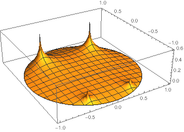
Mathematica graphics

Another example:

poletops = {{-1, 1, 1}, {1, -1, 1}, {0, 0, 3/2}};
rgneqn = (x^2 + y^2)^2 + 8 x y <= 1;
uif = circusTent[poletops, ImplicitRegion[rgneqn, {x, y}], "MaxCellMeasure" -> 0.001]
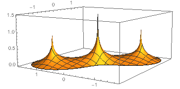
Mathematica graphics

A sleeping version of the OP's request (made with "Operator" -> Laplacian[u[x, y], {x, y}] + a, a between -1 and 2).
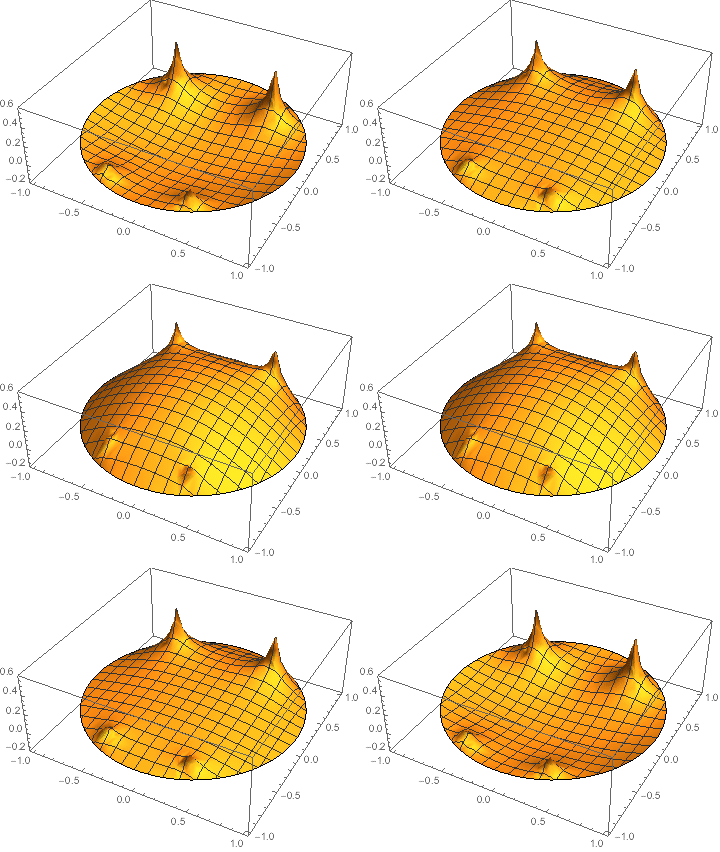
enter image description here

**Edit* - Code for the animation:

movie = Table[ 
   With[{uif = circusTent[icir, Disk[], "Operator" -> Laplacian[u[x, y], {x, y}] + a]},
    Plot3D[uif[x, y], {x, y} ∈ uif["ElementMesh"], 
     PlotRange -> {-0.2, 0.6}, BoxRatios -> Automatic]
    ],
   {a, -1, 2, 0.2}
   ];
movie = Join[movie, Reverse@Most@movie];

Export["1Example.gif", movie]

Also, ToElementMesh uses the global parameter $PerformanceGoal, which has the default setting

If[$ControlActiveSetting, "Speed", "Quality"]

It sometimes fails to produce a mesh when the value is "Speed" (if, say, we replace Table with Manipulate). To use the circusTent in Manipulate or other settings where there are active controls, we need to reset $PerformanceGoal

Manipulate[
 With[{uif = 
    Block[{$PerformanceGoal = "Quality"}, 
     circusTent[icir, Disk[], "Operator" -> Laplacian[u[x, y], {x, y}] + a]]},
  Plot3D[uif[x, y], {x, y} ∈ uif["ElementMesh"], 
   PlotRange -> {-0.2, 0.6}, BoxRatios -> Automatic]
  ],
 {a, -1, 2}
 ]
$\endgroup$
3
  • $\begingroup$ ,Among all the good answers, I have to say this is exactly what I want. And the result is out of my imagination. Mathematica is incredible amazing! By the way, how can I realize the animation as your last photo does. Thank you again. $\endgroup$
    – xibinke
    Commented Nov 10, 2014 at 9:08
  • $\begingroup$ @xibinke You're welcome. I added the code for the animation. Thank you for the accept. $\endgroup$
    – Michael E2
    Commented Nov 10, 2014 at 11:06
  • $\begingroup$ I like you item number 2) :-) $\endgroup$
    – user21
    Commented Jan 23, 2015 at 15:04
7
$\begingroup$

Firstly to use BSplineSurface an array of control points is required, in your case:

Graphics3D[BSplineSurface[Partition[icir, 2]]]

As Öskå commented you can simply use ListPlot3D[icir]. The RegionFunction option will limit the surface to a given region (see below) but your example points all fall within the unit circle so you won't see a circular boundary.

If you want to use a BSpline surface then one way is to define a BSplineFunction using your control points and use that in ParametricPlot3D.

Here is an array of control points for a random surface over the unit square:

cpts = Table[{i, j, RandomReal[{-1, 1}]}, {i, -1, 1, 2/5}, {j, -1, 1, 2/5}];

and a plot the BSplineFunction of these points limited to the unit circle:

ParametricPlot3D[BSplineFunction[cpts][u, v], {u, 0, 1}, {v, 0, 1}, 
   RegionFunction -> (#1^2 + #2^2 <= 1 &)]

ParametricPlot3D

Notice the BSplineFunction parameters, u and v run from 0 to 1.

$\endgroup$
4
$\begingroup$

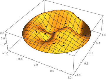
Using J.M.'s implementation of polyharmonic splines:

points = {1, 1, 0.2} # & /@ 
   Select[RandomReal[{-1, 1}, {20, 3}], f @@ Most@# > 0 &];
f[x_, y_] := 1 - x^2 - y^2
pointsByF = ({1, 1, 1/f @@ Most@#} # &) /@ points;
zByF[x_, y_] := Evaluate@polyharmonicSpline[pointsByF, {x, y}];
z[x_, y_] := f[x, y] zByF[x, y]
Show[Plot3D[z[x, y], {x, -1, 1}, {y, -1, 1}, Exclusions -> None, 
  RegionFunction -> (f[#1, #2] >= 0 &)], 
 Graphics3D[{Black, Sphere[points, 0.02]}], BoxRatios -> Automatic, 
 PlotRange -> All]

enter image description here

$\endgroup$
0

Your Answer

By clicking “Post Your Answer”, you agree to our terms of service and acknowledge you have read our privacy policy.

Not the answer you're looking for? Browse other questions tagged or ask your own question.