I seem to have missed this earlier. Anyway, creating a closed spline in Mathematica explicitly is actually rather simple. Witness the following:
pts = {{1, 4}, {.5, 6}, {5, 4}, {3, 12}, {11, 14}, {8, 4}, {12, 3}, {11, 9},
       {15, 10}, {17, 8}};

m = 5; (* degree *) n = Length[pts];
f = BSplineFunction[pts, SplineClosed -> True, SplineDegree -> m];

fn = BSplineFunction[ArrayPad[pts, {{0, m}, {0, 0}}, "Periodic"],
                     SplineDegree -> m,
                     SplineKnots -> ArrayPad[Subdivide[n], m, "Extrapolated"]];
Now, try executingSee the correspondence:
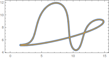
ParametricPlot[{f[t], fn[t]}, {t, 0, 1}, Axes -> None, Frame -> True,
               PlotStyle -> {AbsoluteThickness[6], AbsoluteThickness[2]}]

Further proof of correspondence can be seen by trying ParametricPlot[f[t] - fn[t], {t, 0, 1}]. ;)
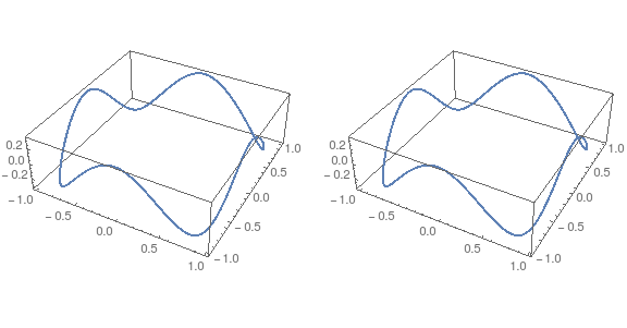
Another example:
pts = {{0, 1, 1}, {1, 1, -1}, {1, 0, 1}, {1, -1, -1}, {0, -1, 1}, {-1, -1, -1},
       {-1, 0, 1}, {-1, 1, -1}};
n = Length[pts];
f = BSplineFunction[pts, SplineClosed -> True];
fn = BSplineFunction[ArrayPad[pts, {{0, 3}, {0, 0}}, "Periodic"],
                     SplineKnots -> ArrayPad[Subdivide[n], 3, "Extrapolated"]];

{ParametricPlot3D[f[t], -{t, fn[t]0, 1}], ParametricPlot3D[fn[t], {t, 0, 1}]}
// GraphicsRow

