Scaled and ImageScaled coordinates are extremely useful to study the behaviors of the options for Graphics. I'll try to contribute what I can. What follows, mostly applies to Plot and similar functions. Often Graphics created explicitly with the Graphics head, such as those in Mr.Wizard's answer may behave differently, as compared to Plot.

First example:

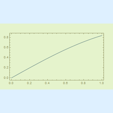
Plot[Sin[x], {x, 0, 1},
     Frame -> True, Background -> LightBlue, 
     AspectRatio -> 0.5, ImageSize -> {360, 360},
     ImagePadding -> 30, PlotRangeClipping -> False, 
     Epilog -> {Opacity[.2], Yellow, 
                Rectangle[ImageScaled[{0, 0}],
                          ImageScaled[{1, 1}]
                         ]
               }
    ]

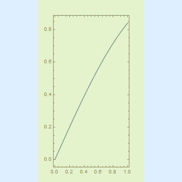
Show[%, AspectRatio -> 2]

ImageDimensions @ %%
ImageDimensions @ %%

{360, 360}
{360, 360}

Conflicting specifications for ImageSize and AspectRatio lead to a plot, that is as large as possible, while conforming to AspectRatio and not exceeding the ImageSize. I find especially peculiar the fact, that ImageScaled[{0,0}] is at the boundary of the padding of the image, not the lower-left corner of the entire graphic. This is illustrated by the translucent yellow rectangle, which occupies the ImageScaled range from {0,0} to {1,1}, while the light-blue background covers the entire {360, 360} square.

As Alexey pointed out, the accurate description of AspectRatio's behavior is hidden quite deep in the documentation, specifically under the "Properties and Relations" tab.

AspectRatio determines the ratio of PlotRange, not ImageSize.

This is easily tested with the rasterize trick, similar to what Alexey did in the linked question.

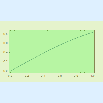
g = 
Plot[Sin[x], {x, 0, 1},
     Frame -> True, Background -> LightBlue, 
     AspectRatio -> 0.5, ImageSize -> {360, 360},
     ImagePadding -> 30, PlotRangeClipping -> False, 
     Epilog -> {Opacity[.2], Yellow, 
                Rectangle[ImageScaled[{0, 0}],
                          ImageScaled[{1, 1}]
                         ],
                Green,
                Annotation[Rectangle[Scaled[{0, 0}],
                                     Scaled[{1, 1}]
                                    ],
                           "One", "Region"
                          ]
               }
    ]

The green rectangle is annotated and covers the PlotRange, as per definition of Scaled. I use Rasterize to get the coordinate range it occupies in terms of printer points:

Rasterize[g, "Regions"]

{{"One", "Region"} -> {{30., 105.}, {330., 255.}}}

This output means, that the annotated rectangle occupies pixels lying in the range from {30., 105.} to {330., 255.}. These are Real numbers, by the way, not integers. Rasterize in this respect is very accurate and can calculate sizes to three digits past the decimal, unlike, say, ImageDimensions which returns integers. Also, when using this trick for other needs, it's very important to remember, that the coordinates in the rasterized graphics are flipped. x is zero on the left, as usual, but y=0 is located at the top of the image.

Table[#2/#1 & @@ (#2 - #1) & @@ 
  Rasterize[Show[g, AspectRatio -> i], "Regions"][[-1, 2]], {i, .1, 1.9, .1}]

{0.1, 0.2, 0.3, ... , 1.7, 1.8, 1.9}

That much we knew. The plot range or, in other words, the Scaled[{0,0}] to Scaled[{1,1}] ranges conforms to the AspectRatio. Show is convenient in allowing us to override any of the options of g. Therefore we can study effects of altering PlotRangePadding and others:

Table[#2/#1 & @@ (#2 - #1) & @@ 
  Rasterize[Show[g, AspectRatio -> i,
                    PlotRangePadding -> 1,
                    ImagePadding -> {{150, 6}, {100, 20}}],
            "Regions"][[-1, 2]], {i, .1, 1.9, .1}]

However, the output remains the same. This can be easily expanded to a Dynamic or Manipulate construct, but I feel that "AspectRatio controls the height-to-width of the PlotRange" is a sufficiently exhaustive description.